- New to JMP? Let the Data Analysis Director guide you through selecting an analysis task, an analysis goal, and a data type. Available now in the JMP Marketplace!
- See how to install JMP Marketplace extensions to customize and enhance JMP.
- Subscribe to RSS Feed
- Mark Topic as New
- Mark Topic as Read
- Float this Topic for Current User
- Bookmark
- Subscribe
- Mute
- Printer Friendly Page
Discussions
Solve problems, and share tips and tricks with other JMP users.- JMP User Community
- :
- Discussions
- :
- Re: Matching comparison of two samples doesn't make sense
- Mark as New
- Bookmark
- Subscribe
- Mute
- Subscribe to RSS Feed
- Get Direct Link
- Report Inappropriate Content
Matching comparison of two samples doesn't make sense
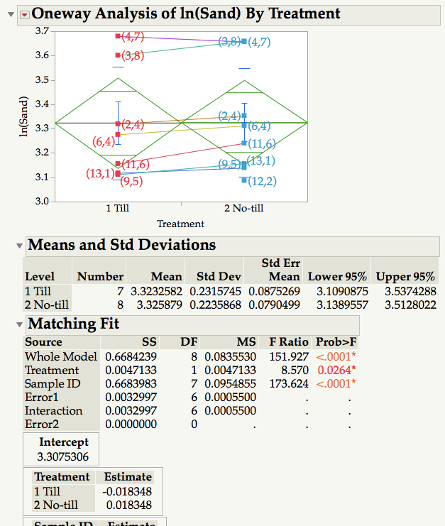
I ran a matching comparison between two sets of measurements (Platform: Fit Y by X) using Sample ID as matching variable and Treatment as grouping variable. Obviously, the objective is to see if Treatment has an effect on the dependent variable. Results show that Treatment is significant (p = 0.03) whereas the mean diamonds and common sense indicate it is not. Omiting the non-matching observation (12,2) from the No-till treatment so that both samples have 7 measurements does not change the result. What am I missing?
Accepted Solutions
- Mark as New
- Bookmark
- Subscribe
- Mute
- Subscribe to RSS Feed
- Get Direct Link
- Report Inappropriate Content
Re: Matching comparison of two samples doesn't make sense
There are several methods to complete a matched pair, or paired analysis in JMP. The Anova Matched Pairs analysis displays the data with its own scale. The largest effect in your model is Sample ID (or block). After removing the Sample ID effect, the average difference in the Till methods is 0.036696 = (0.018348 - -0.018348). The Sum of Squares, SS, of the differences is 0.0047133 (since there is only 1 degree of freedom, this is also the MS). And the MS error is 0.00055 ( the sqrt is an estimate of the std dev of the differences). The F ratio with 1 and 6 degree of freedom is 8.56963 (8.570) which is statisticially different from zero.
The reason the treatment effect is not visible in your display is because the ID variability is more than 100x of the treatment effect. Below I'll document a couple of alternate methods, which depend upon how you table is organized.
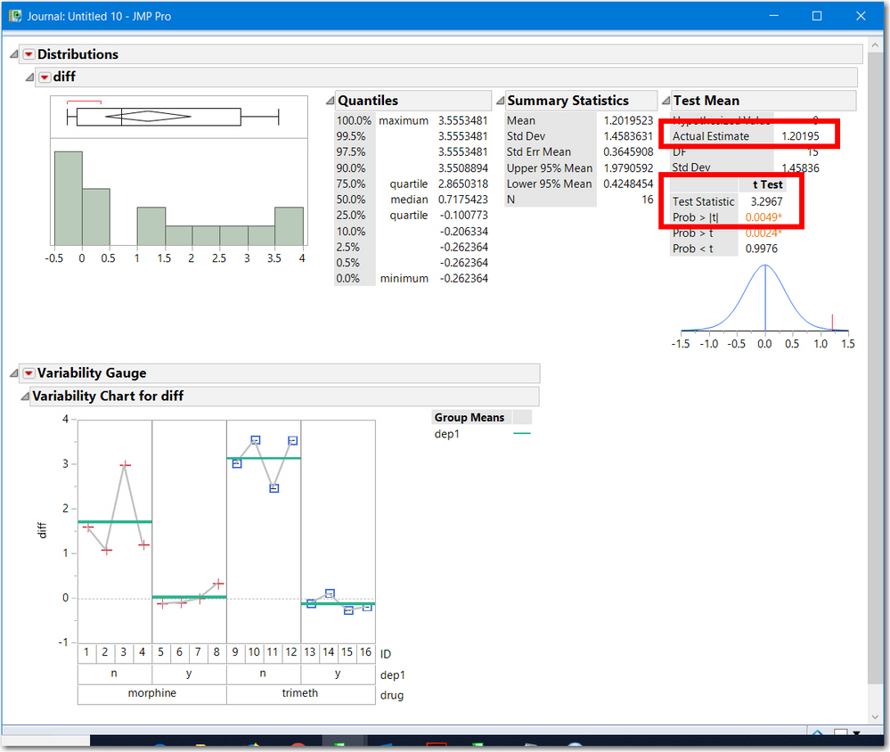
- Each row represents a pair with 2 columns, 1-Till and No-Till. (This is often called the paired/mulivariate/correlation layout. Compute the difference and analyze the differences to test if equivalent to zero. I like to plot the differences by ID and use Distribution to test if the difference is zero.
- Same table layout, use Fit Y by X use No-Till for Y and 1-Till for X. Then request a paired t-test. To do this, hold down the SHIFT key then select the red menu, and the paired t-test option is visible.
- Table is stacked, with a column for Sample ID and another for Treatment. (This is often called the ANOVA layout). Use Analyze Fit Y by X, Y is the response and X is the treatment, then select matched pairs and select the ID column. This is what you used.
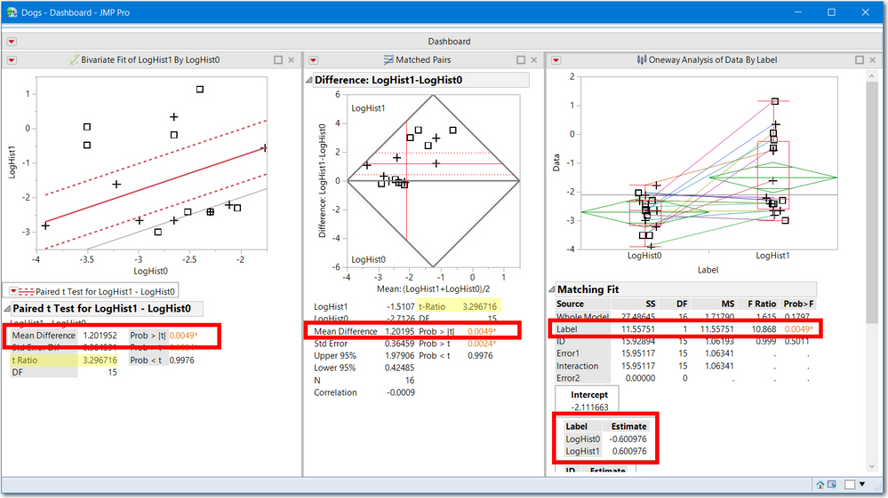
I do not have your data so I will use Dogs.jmp to demonstrate the 3 JMP platform methods displayed in a single dashboard. Note:
- all three have the same statistical significance 0.0049
- two use the t-test (3.29676) and the third is an F ratio (10.868) which is the square of t. An F with (1, df) degrees of freedom is the square of a t statistic with df degrees of freedom.
- the average difference (1.20195) is equal to the difference of the 2 treatment estimates.
- the 3rd analysis was achieved by stacking LogHist0 and LogHist1 the stacked column is called Data and the variable name is called Label.
- The first two methods show a gray line, representing the test: the line Y==X and Diff==0. Both are outside the 95% confidence intervals, hence statistically significant.
All of these graphs are in the original scale of the Dogs.jmp sample data, which is okay since the treatment effect is larger that the ID (blocking) effect. However, these pictures still are not my preferred display. See below. 
For your data split the response by treatment and use ID for grouping. Compute the paired differences. And run the Distribution and Diff by ID graph. Another approach is to create a new column with the formula to compute response mean by ID (the ID means). Then compute the response minus the ID average. I call this block aligned data. Use this data for your matched pairs differences, with the two means diamonds, etc. (You would not have to split your table).
I hope the mini-statistics lecture was helpful.
Oh one last comment while the test was statistially different frm zero, the question is whether the average difference is of practical importance to your work.
- Mark as New
- Bookmark
- Subscribe
- Mute
- Subscribe to RSS Feed
- Get Direct Link
- Report Inappropriate Content
Re: Matching comparison of two samples doesn't make sense
Yes, to both your questions, if the there are no violations of assumptions. I still recommend you look at the differences by ID.
Like the Dogs.jmp data you might find the difference to be large for a subset of subjects/units and nothing for another group. In my opinion, too little attention is spent on checking the randomness assumptions and hence not looking for other factors that might be causing the inconsistencies. For simplicity, I like to call it a block* treatment interaction, but mostly it is another (unkown) factor.
Good Luck!
- Mark as New
- Bookmark
- Subscribe
- Mute
- Subscribe to RSS Feed
- Get Direct Link
- Report Inappropriate Content
Re: Matching comparison of two samples doesn't make sense
There are several methods to complete a matched pair, or paired analysis in JMP. The Anova Matched Pairs analysis displays the data with its own scale. The largest effect in your model is Sample ID (or block). After removing the Sample ID effect, the average difference in the Till methods is 0.036696 = (0.018348 - -0.018348). The Sum of Squares, SS, of the differences is 0.0047133 (since there is only 1 degree of freedom, this is also the MS). And the MS error is 0.00055 ( the sqrt is an estimate of the std dev of the differences). The F ratio with 1 and 6 degree of freedom is 8.56963 (8.570) which is statisticially different from zero.
The reason the treatment effect is not visible in your display is because the ID variability is more than 100x of the treatment effect. Below I'll document a couple of alternate methods, which depend upon how you table is organized.
- Each row represents a pair with 2 columns, 1-Till and No-Till. (This is often called the paired/mulivariate/correlation layout. Compute the difference and analyze the differences to test if equivalent to zero. I like to plot the differences by ID and use Distribution to test if the difference is zero.
- Same table layout, use Fit Y by X use No-Till for Y and 1-Till for X. Then request a paired t-test. To do this, hold down the SHIFT key then select the red menu, and the paired t-test option is visible.
- Table is stacked, with a column for Sample ID and another for Treatment. (This is often called the ANOVA layout). Use Analyze Fit Y by X, Y is the response and X is the treatment, then select matched pairs and select the ID column. This is what you used.
I do not have your data so I will use Dogs.jmp to demonstrate the 3 JMP platform methods displayed in a single dashboard. Note:
- all three have the same statistical significance 0.0049
- two use the t-test (3.29676) and the third is an F ratio (10.868) which is the square of t. An F with (1, df) degrees of freedom is the square of a t statistic with df degrees of freedom.
- the average difference (1.20195) is equal to the difference of the 2 treatment estimates.
- the 3rd analysis was achieved by stacking LogHist0 and LogHist1 the stacked column is called Data and the variable name is called Label.
- The first two methods show a gray line, representing the test: the line Y==X and Diff==0. Both are outside the 95% confidence intervals, hence statistically significant.
All of these graphs are in the original scale of the Dogs.jmp sample data, which is okay since the treatment effect is larger that the ID (blocking) effect. However, these pictures still are not my preferred display. See below. 
For your data split the response by treatment and use ID for grouping. Compute the paired differences. And run the Distribution and Diff by ID graph. Another approach is to create a new column with the formula to compute response mean by ID (the ID means). Then compute the response minus the ID average. I call this block aligned data. Use this data for your matched pairs differences, with the two means diamonds, etc. (You would not have to split your table).
I hope the mini-statistics lecture was helpful.
Oh one last comment while the test was statistially different frm zero, the question is whether the average difference is of practical importance to your work.
- Mark as New
- Bookmark
- Subscribe
- Mute
- Subscribe to RSS Feed
- Get Direct Link
- Report Inappropriate Content
Re: Matching comparison of two samples doesn't make sense
I hope the mini-statistics lecture was helpful.
Oh one last comment while the test was statistially different frm zero, the question is whether the average difference is of practical importance to your work.
Yes, a bit dense, but helpful. Thank you.
Am I correct in saying that, based on the p=0.03 of the F statistic for Treatment, the Treatment effect is small, albeit statistically significant at α=0.05?
Is it also fair to say that, had the analysis been conducted on unmatched pairs, the Treatment effect would not be statistically significant?
Whether the difference is of practical importance, yes it is, because it concerns a long term experiment. The difference may look small to you this year. I expect it to be bigger next year, and so on.
Cheers
- Mark as New
- Bookmark
- Subscribe
- Mute
- Subscribe to RSS Feed
- Get Direct Link
- Report Inappropriate Content
Re: Matching comparison of two samples doesn't make sense
Yes, to both your questions, if the there are no violations of assumptions. I still recommend you look at the differences by ID.
Like the Dogs.jmp data you might find the difference to be large for a subset of subjects/units and nothing for another group. In my opinion, too little attention is spent on checking the randomness assumptions and hence not looking for other factors that might be causing the inconsistencies. For simplicity, I like to call it a block* treatment interaction, but mostly it is another (unkown) factor.
Good Luck!
Recommended Articles
- © 2026 JMP Statistical Discovery LLC. All Rights Reserved.
- Terms of Use
- Privacy Statement
- Contact Us

