JMP Support Vector Machines (SVM) platform

[#1]

I am trying to recreate SVM model I did in R but now using JMP builtin SVM platform. Is it possible to do JMP SVM without scaling and centering of my input parameters? I have chemical mixture components expressed in weight fractions so all of them have the same units (wt.fractions). I also wonder if JMP SVM can optimize C and Gamma or I need to do it in R? I am using JMP Pro 15.0.

[#2 · Accepted solution]

I don't see any way to turn off the centering and scaling. If all of the inputs are on the same scale, the centering and scaling will not really change that. It affects the "parameters" of the model, but not the model that results. In other words, it won't matter if they are on a 0 to 1 scale or a -1 to +1 scale. The relationships among the X's will remain the same.

As for C and Gamma, from the JMP documentation: 

Tip: To find the best fitting model, fit a range of kernel functions and parameter values and use the Model Comparison report.

So, JMP will not optimize these parameters for you. One could imagine writing a JMP script to do this, but the script may take some time to run since it needs to fit the SVM for multiple combinations of C and Gamma,and then you would still likely need to do some form of interpolation (or model-building) to find the "optimum".

[#3 · Accepted solution]

Here's a quick example of iterating through a range of parameters.  no finesse, just brute force.

Note, that after the report comes up, the best model is indicated in the report comparison.

dt=Open("$SAMPLE_DATA/Big Class.jmp")

gam=.1;
cos=.5;

dt<<obj=	Support Vector Machines(
	Y( :age ),
	X( :height, :weight ),
	Fit(
		Kernel Function( "Radial Basis Function" ),
		Gamma( gam ),
		Cost( cos ),
		Validation Method( "None" ),
	)
);
for(i=1, i<=10, i++,
	for (ii=1, ii<=10, ii++,
		
		
	obj<<Fit(
		Kernel Function( "Radial Basis Function" ),
		Gamma( gam ),
		Cost( cos ),
		Validation Method( "None" )
	);	
	gam=gam+.1);
	cos=cos+.5
);

[#4]

it gives an error like this:
attempting to assign to an object that is not an L-value in access or evaluation of 'Assign' , dt << obj = /*###*/Support Vector Machines(
Y( :age ),
X( :height, :weight ),
Fit(
Kernel Function( "Radial Basis Function" ),
Gamma( gam ),
Cost( cos ),
Validation Method( "None" )
)
) /*###*/

What did I do wrong?

[#5]

I changed it a bit and it works, thanks!

dt = Open( "$SAMPLE_DATA/Big Class.jmp" );

gam = .1;
cos = .5;

svm = dt << Support Vector Machines(
	Y( :age ),
	X( :height, :weight ),
	Fit( Kernel Function( "Radial Basis Function" ), Gamma( gam ), Cost( cos ), Validation Method( "None" ), )
);

For( i = 1, i <= 10, i++,
	For( ii = 1, ii <= 10, ii++, 
		svm << Fit(
			Kernel Function( "Radial Basis Function" ),
			Gamma( gam ),
			Cost( cos ),
			Validation Method( "None" )
		);
		gam = gam + .1;
	);
	cos = cos + .5;
);

[#6 · Accepted solution]

I changed it a bit, too. Mostly a matter of personal style.

Names Default to Here( 1 );

// use a small example
data = Open( "$SAMPLE_DATA/Big Class.jmp" );

// launch SVM platform
svm = data << Support Vector Machines(
	Y( :age ),
	X( :height, :weight )
);

// iterate over a range of hyper-parameters
For( cost = 0.5, cost <= 5, cost += 0.5,
	For( gamma = 0.1, gamma <= 1, gamma += 0.1, 
		svm << Fit(
			Kernel Function( "Radial Basis Function" ),
			Gamma( gamma ),
			Cost( cost ),
			Validation Method( "None" )
		);
	);
);

// separate parameters and performance in a new table
results = Report( svm )["Model Comparison"][TableBox(1)] << Make Into Data Table;

// fit interpolator for profiling
results << Neural(
	Y( :Training Misclassification Rate ),
	X( :Cost, :Gamma ),
	Informative Missing( 0 ),
	Validation Method( "Holdback", 0.3333 ),
	Fit(
		NTanH( 3 ),
		Profiler(
			1,
			Confidence Intervals( 1 ),
			Term Value(
				Cost( 2.75, Lock( 0 ), Show( 1 ) ),
				Gamma( 1, Lock( 0 ), Show( 1 ) )
			)
		),
		Plot Actual by Predicted( 1 ),
		Plot Residual by Predicted( 1 )
	)
);

But I also added another step to understand how the miss-classification rate depended on the hyper-parameters. I saved the table from Model Comparison and fit a simple (but adequate) neural network. The profiler can be used to find good values and understand them. For example, using a high gamma and a moderate cost with little improvement by increasing the cost.

[#7]

How can I force Probability Threshold to stay 0.5 all time?
When I run Cost and Gamma optimization using Validation Method("KFold", 10), it always calculates Validation Misclassification using adjusted threshold, so it calculates Conditional Validation Misclassification Rate, please see attached file. I can not select best Cost and Gamma as there is third parameter Threshold that I am not trying to optimize.

[#8]

I also using JMP Pro 15.0.Try Machines (SVM) .Thanks!

[#9]

Hi @Mark_Bailey,

  Is there a benefit of using the NN platform for finding the optimal settings for the cost and gamma?

  I do something similar with my data to find optimal hyperparameter settings, but instead of using the NN to try and find the optimal, I use the Gaussian Process platform. I compared the fits from each of the two "optimal" options and the one from the Gaussian Process had a misclassification rate of 0.25 vs 0.275 for the NN method.

Snap1.png

 

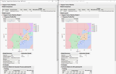
Just curious.

Thanks!,

DS

[#10]

The questions were about the hyper-parameters for the Neural fitting process. We were not using a Neural model of results from another platform hyper-parameters.