Is JMP miscalculating my RMSE

[#1]

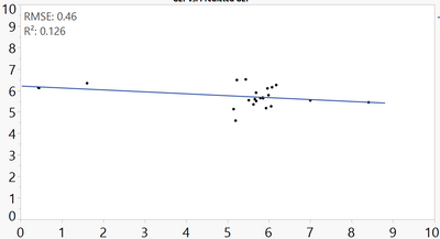
I plotted my observed vs predicted values, and added a line of fit with the RMSE, however, the values it's calculating/displaying is significantly lower than what I'm calculating and expecting (0.46 vs 2.07).

Here's the data:

6.343	1.607119
6.259	6.177004
6.139	0.429539
5.266	6.05368
5.451	8.40834
6.492	5.226375
6.52	5.440272
5.784	5.990638
6.154	6.07527
6.103	5.965431
6.122	0.445846
5.541	7.000725
5.181	5.931456
5.355	5.626706
5.674	5.849083
5.642	5.859607
5.136	5.14744
5.512	5.693088
5.9	5.690088
5.65	5.792552
5.55	5.513773
5.6	5.659517
4.6	5.195817

Am I missing something?

[#2]

Welcome to the community.  

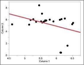
I'm not sure what you are trying to do.  In the data set you show, is column 1 the actual values and column 2 the predicted values?  The difference in these is called the residuals.  

I don't see what you are trying to model?  Typically, you will have at least 1 independent variable and at least 1 dependent variable and the RMSE is the standard deviation of the model fit.  I don't know which is which in your data set?  But if you were modeling these 2 columns, I get completely different results than you?

There are many ways to look at residuals for the main purpose of determining if your model meets the fundamental assumptions of quantitative analysis (NID(0, variance)). 

Summary of Fit
RSquare
0.125645
RSquare Adj
0.084009
Root Mean Square Error
1.804222
Mean of Response
5.251277
Observations (or Sum Wgts)
23

[#3]

@statman

I noticed this interesting calculation as well when I used Python to model my experiment. I run a model, JMP gives me a RMSE, and then I save column of the predicted value. I used the formula below to do calculation in Excel, which gives me a different RMSE result with JMP. Could you please tell what's wrong for my calculation?

[#4]

Simple question: do you take the square root of the MSE then to obtain the RMSE?

[#5]

I just realized I made a mistake by ignoring df. The formula above is not right, should divide by degree of residuals instead of n, and then square root of it.

[#6]

The error degrees of freedom equal the number of observations (23) minus the number of parameters estimated (2). This script shows how you can calculate the RMSE and compares it to the result from the Bivariate platform. I'm curious why you calculate RMSE with Excel when JMP gives you the answer.

Names Default to Here( 1 );

// duplicate example in discussion
dt = New Table( "RMSE Example",
	Add Rows( 23 ),
	New Script(
		"Source",
		Open(
			"https://community.jmp.com/t5/Discussions/Is-JMP-miscalculating-my-RMSE/m-p/583546",
			HTML Table( 1, Column Names( 0 ), Data Starts( 1 ) )
		)
	),
	New Column( "X",
		Numeric,
		"Continuous",
		Format( "Best", 12 ),
		Set Values(
			[6.343, 6.259, 6.139, 5.266, 5.451, 6.492, 6.52, 5.784, 6.154, 6.103,
			6.122, 5.541, 5.181, 5.355, 5.674, 5.642, 5.136, 5.512, 5.9, 5.65, 5.55,
			5.6, 4.6]
		)
	),
	New Column( "Y",
		Numeric,
		"Continuous",
		Format( "Best", 12 ),
		Set Values(
			[1.607119, 6.177004, 0.429539, 6.05368, 8.40834, 5.226375, 5.440272,
			5.990638, 6.07527, 5.965431, 0.445846, 7.000725, 5.931456, 5.626706,
			5.849083, 5.859607, 5.14744, 5.693088, 5.690088, 5.792552, 5.513773,
			5.659517, 5.195817]
		)
	)
);

// calculate RMSE with Bivariate platform
obj = Bivariate( Y( :Y ), X( :X ), Fit Line( 1 ) );
bivRMSE = (obj << Report)["Summary of Fit"][NumberColBox(1)] << Get( 3 );

// calculate RMSE uing direct linear regression
yData = dt:Y << Get As Matrix;
xData = dt:X << Get As Matrix;
{ estimate, se, diagnostic } = Linear Regression( yData, xData );
predY = estimate[1] + estimate[2] * xData;
df = N Row( yData ) - 2;	// error df = n - 2 for parameter estimates
manRMSE = Sqrt( Sum( (yData - predY)^2 ) / df );

// compare results
Show( bivRMSE, manRMSE );

[#7]

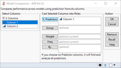
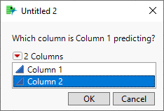
Expanding on @statman's comments and assuming you were trying to predict the first column from the second, it looks like you fit your residuals with a second linear model.  This would mean you created a type of ensemble model from whatever your first model was and a linear term.  This would further reduce your error, giving you a smaller RMSE.  I believe instead you likely wanted to use the Model Comparison platform under Analyze > Predictive Modeling > Model Comparison.

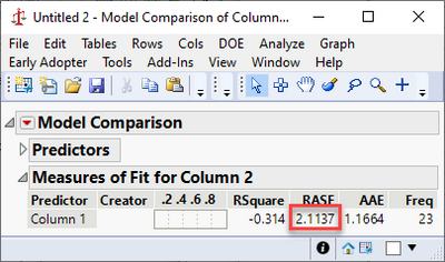
This gives a reported RASE that is closer to your expected RMSE.

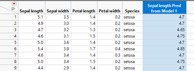
As an example, consider the iris sample data set.  If you use some method to predict Sepal length and predict it to be a function of Sepal length as shown in the equation below, you will get a reasonable model.

But, the slope, or parameter estimate for Sepal width, is not quite right (or at least it does not match what is observed in the data).  

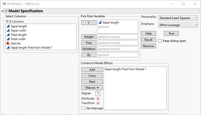
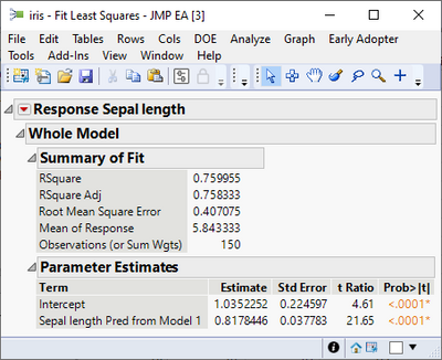
Thus, you can fit a second model from the output of the first using a linear model to improve the fit (this is because there is a pattern in the residuals).

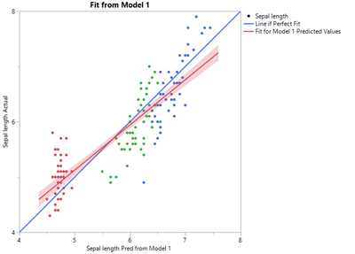
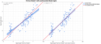
Saving the predicted formula gives a new predicted formula column based on another predicted formula column. Note how the slope of the blue line changes.

In this case you will get the same result as if you just modeled Sepal length from Petal length using a linear model, but that would not always be true depending on what was used for the first model.

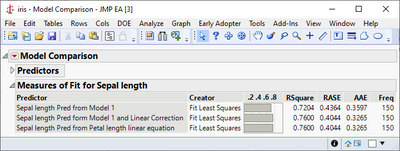
Brining up the Model Comparison shows the improvement from the second model:

This should recreate the iris graphs:

View more...

Names default to here(1);

dt = Open("$Sample_data/iris.jmp");

dt << New Column("Sepal length Pred from Model 1", Numeric, "Continuous", Format("Best", 12), Set Property("Notes", "Prediction Formula"), Set Property("Predicting", {:Sepal length, Creator("Fit Least Squares")}), Formula(4 + 0.5 * :Petal length), Set Display Width(129));
dt << New Column("Sepal length Pred form Model 1 and Linear Correction", Numeric, "Continuous", Format("Best", 12), Set Property("Notes", "Prediction Formula"), Formula(1.03522519623809 + 0.817844554702371 * :Sepal length Pred from Model 1), Set Property("Predicting", {:Sepal length, Creator("Fit Least Squares")}));
dt << New Column("Sepal length Pred from Petal length linear equation", Numeric, "Continuous", Format("Best", 12), Set Property("Notes", "Prediction Formula"), Formula(4.30660341504758 + 0.408922277351185 * :Petal length), Set Property("Predicting", {:Sepal length, Creator("Fit Least Squares")}));

dt << Graph Builder(
	Size( 473, 500 ),
	Variables(
		X( :Sepal length Pred from Model 1 ),
		Y( :Sepal length ),
		Y(
			Transform Column(
				"Transform[Sepal...d from Model 1]",
				Formula( :Sepal length Pred from Model 1 )
			),
			Position( 1 )
		)
	),
	Elements(
		Points( X, Y( 1 ), Legend( 5 ) ),
		Formula( X, Y( 2 ), Legend( 7 ) ),
		Line Of Fit( X, Y( 1 ), Legend( 9 ) )
	),
	SendToReport(
		Dispatch( {"Line Of Fit"}, "", OutlineBox, {Close( 0 )} ),
		Dispatch(
			{},
			"Sepal length Pred from Model 1",
			ScaleBox,
			{Min( 4 ), Max( 8 ), Inc( 1 ), Minor Ticks( 1 )}
		),
		Dispatch(
			{},
			"Sepal length",
			ScaleBox,
			{Min( 4 ), Max( 8 ), Inc( 2 ), Minor Ticks( 1 )}
		),
		Dispatch(
			{},
			"400",
			ScaleBox,
			{Legend Model(
				7,
				Level Name(
					0,
					"Line if Perfect Fit",
					Item ID( "Transform[Sepal...d from Model 1]", 1 )
				)
			), Legend Model(
				9,
				Level Name(
					0,
					"Fit for Model 1 Predicted Values",
					Item ID( "Sepal length", 1 )
				)
			)}
		),
		Dispatch( {}, "graph title", TextEditBox, {Set Text( "Fit from Model 1" )} ),
		Dispatch( {}, "Y title", TextEditBox, {Set Text( "Sepal length Actual" )} )
	)
);

dt << Fit Model(
	Y( :Sepal length Pred form Model 1 and Linear Correction ),
	Effects( :Sepal length ),
	Personality( "Standard Least Squares" ),
	Emphasis( "Effect Leverage" ),
	Run(
		:Sepal length Pred form Model 1 and Linear Correction <<
		{Summary of Fit( 1 ), Analysis of Variance( 1 ), Parameter Estimates( 1 ),
		Scaled Estimates( 0 ), Plot Actual by Predicted( 1 ),
		Plot Residual by Predicted( 1 ), Plot Studentized Residuals( 0 ),
		Plot Effect Leverage( 1 ), Plot Residual by Normal Quantiles( 0 ),
		Box Cox Y Transformation( 0 )}
	)
);

dt << Graph Builder(
	Size( 949, 500 ),
	Variables(
		X( :Sepal length Pred from Model 1 ),
		X( :Sepal length Pred form Model 1 and Linear Correction ),
		Y( :Sepal length ),
		Y(
			Transform Column(
				"Transform[Sepal...d from Model 1]",
				Formula( :Sepal length Pred from Model 1 )
			),
			Position( 1 )
		),
		Y(
			Transform Column(
				"Transform[Sepal...inear equation]",
				Formula( :Sepal length Pred from Petal length linear equation )
			),
			Position( 1 )
		),
		Y(
			Transform Column(
				"Transform[Sepal...inear equation]",
				Formula( :Sepal length Pred from Petal length linear equation )
			),
			Position( 1 )
		),
		Y(
			Transform Column(
				"Transform[Sepal...ear Correction]",
				Formula( :Sepal length Pred form Model 1 and Linear Correction )
			),
			Position( 1 )
		)
	),
	Elements(
		Position( 1, 1 ),
		Points( X, Y( 1 ), Legend( 5 ) ),
		Line Of Fit(
			X,
			Y( 1 ),
			Legend( 9 ),
			Root Mean Square Error( 1 ),
			Equation( 1 )
		),
		Formula( X, Y( 2 ), Legend( 7 ) )
	),
	Elements(
		Position( 2, 1 ),
		Points( X, Y( 1 ), Legend( 10 ) ),
		Line Of Fit( X, Y( 1 ), Legend( 12 ), Equation( 1 ) ),
		Formula( X, Y( 5 ), Legend( 13 ) )
	),
	SendToReport(
		Dispatch(
			{},
			"Sepal length Pred from Model 1",
			ScaleBox,
			{Min( 4 ), Max( 8 ), Inc( 1 ), Minor Ticks( 3 ),
			Label Row( {Show Major Grid( 1 ), Show Minor Grid( 1 )} )}
		),
		Dispatch(
			{},
			"Sepal length Pred form Model 1 and Linear Correction",
			ScaleBox,
			{Min( 4 ), Max( 8 ), Inc( 1 ), Minor Ticks( 3 ),
			Label Row( {Show Major Grid( 1 ), Show Minor Grid( 1 )} )}
		),
		Dispatch(
			{},
			"Sepal length",
			ScaleBox,
			{Min( 4 ), Max( 8 ), Inc( 1 ), Minor Ticks( 3 ),
			Label Row( {Show Major Grid( 1 ), Show Minor Grid( 1 )} )}
		),
		Dispatch(
			{},
			"400",
			ScaleBox,
			{Legend Model(
				5,
				Level Name( 0, "Actual Value", Item ID( "Sepal length", 1 ) ),
				Base( 0, 0, 0, Item ID( "Sepal length", 1 ) ),
				Properties( 0, {Line Color( 21 )}, Item ID( "Sepal length", 1 ) )
			), Legend Model(
				9,
				Level Name(
					0,
					"Fit line from predicted values",
					Item ID( "Sepal length", 1 )
				),
				Properties( 0, {Line Color( 21 )}, Item ID( "Sepal length", 1 ) )
			), Legend Model(
				7,
				Level Name(
					0,
					"Fit if perfect model",
					Item ID( "Transform[Sepal...d from Model 1]", 1 )
				),
				Properties(
					0,
					{Line Color( 3 )},
					Item ID( "Transform[Sepal...d from Model 1]", 1 )
				)
			), Legend Model(
				10,
				Properties( 0, {Line Color( 21 )}, Item ID( "Sepal length", 1 ) )
			), Legend Model(
				12,
				Properties( 0, {Line Color( 21 )}, Item ID( "Sepal length", 1 ) )
			), Legend Model(
				13,
				Properties(
					0,
					{Line Color( 3 )},
					Item ID( "Transform[Sepal...ear Correction]", 1 )
				)
			)}
		),
		Dispatch(
			{},
			"graph title",
			TextEditBox,
			{Set Text( "Fit from Model 1 (left) and Ensemble Model (right)" )}
		),
		Dispatch( {}, "Y title", TextEditBox, {Set Text( "Sepal length Actual" )} ),
		Dispatch(
			{},
			"400",
			LegendBox,
			{Legend Position(
				{5, [0], 9, [1, -3], 7, [2], 10, [-1], 12, [-1, -3], 13, [-1]}
			)}
		)
	)
);

dt << Model Comparison(
	Y(
		:Sepal length Pred from Model 1,
		:Sepal length Pred form Model 1 and Linear Correction,
		:Sepal length Pred from Petal length linear equation
	)
);