- New to JMP? Let the Data Analysis Director guide you through selecting an analysis task, an analysis goal, and a data type. Available now in the JMP Marketplace!
- See how to install JMP Marketplace extensions to customize and enhance JMP.
- Subscribe to RSS Feed
- Mark Topic as New
- Mark Topic as Read
- Float this Topic for Current User
- Bookmark
- Subscribe
- Mute
- Printer Friendly Page
Discussions
Solve problems, and share tips and tricks with other JMP users.- JMP User Community
- :
- Discussions
- :
- Re: How to use JSL to find X variable range to meet spec limit by fixing other v...
- Mark as New
- Bookmark
- Subscribe
- Mute
- Subscribe to RSS Feed
- Get Direct Link
- Report Inappropriate Content
How to use JSL to find X variable range to meet spec limit by fixing other variables in Prediction Profiler?
Hi JSL experts,
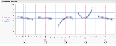
I have a DoE OLS or REML model with prediction profiler like below. How I can find all the X variable ranges to meet LSL and USL automatically with JSL by fixing other variables? For example, X1 must be below 34.6 to meet spec. Thank you so much for your help.
Accepted Solutions
- Mark as New
- Bookmark
- Subscribe
- Mute
- Subscribe to RSS Feed
- Get Direct Link
- Report Inappropriate Content
Re: How to use JSL to find X variable range to meet spec limit by fixing other variables in Prediction Profiler?
I think that there is a more elegant and robust approach. See the end of this example for the approach of which I am thinking.
Names Default to Here( 1 );

// JMP Pro 16.2

// start with example of a model script
model = Expr(
	Fit Group(
		Fit Model(
			Y( :"SILICA (%)"n ),
			Effects( :ELONG, :"HARDNESS(+/-0.2)"n ),
			Personality( "Standard Least Squares" ),
			Emphasis( "Minimal Report" ),
			Run(
				Profiler(
					1,
					Confidence Intervals( 1 ),
					Term Value(
						ELONG( 417.5, Lock( 0 ), Show( 1 ) ),
						"HARDNESS(+/-0.2)"n( 69.775, Lock( 0 ), Show( 1 ) )
					)
				),
				:"SILICA (%)"n << {Summary of Fit( 1 ), Analysis of Variance( 1 ),
				Parameter Estimates( 1 ), Effect Tests( 0 ), Effect Details( 0 ),
				Lack of Fit( 0 ), Scaled Estimates( 0 ), Plot Actual by Predicted( 1 ),
				Plot Regression( 0 ), Plot Residual by Predicted( 0 ),
				Plot Studentized Residuals( 1 ), Plot Effect Leverage( 0 ),
				Plot Residual by Normal Quantiles( 1 ), Box Cox Y Transformation( 0 ),
				Press( 1 )}
			)
		),
		Fit Model(
			Y( :SILANE Value ),
			Effects(
				:"ABRASION For example (%)"n, :MODULUS, :ELONG, :"HARDNESS(+/-0.2)"n,
				:MODULUS * :ELONG
			),
			Personality( "Standard Least Squares" ),
			Emphasis( "Minimal Report" ),
			Run(
				Profiler(
					1,
					Confidence Intervals( 1 ),
					Term Value(
						"ABRASION For example (%)"n( 133.1, Lock( 0 ), Show( 1 ) ),
						MODULUS( 1255, Lock( 0 ), Show( 1 ) ),
						ELONG( 417.5, Lock( 0 ), Show( 1 ) ),
						"HARDNESS(+/-0.2)"n( 69.775, Lock( 0 ), Show( 1 ) )
					)
				),
				:SILANE Value << {Summary of Fit( 1 ), Analysis of Variance( 1 ),
				Parameter Estimates( 1 ), Effect Tests( 0 ), Effect Details( 0 ),
				Lack of Fit( 0 ), Scaled Estimates( 0 ), Plot Actual by Predicted( 1 ),
				Plot Regression( 0 ), Plot Residual by Predicted( 0 ),
				Plot Studentized Residuals( 1 ), Plot Effect Leverage( 0 ),
				Plot Residual by Normal Quantiles( 1 ), Box Cox Y Transformation( 0 ),
				Press( 1 )}
			)
		),
		Fit Model(
			Y( :SULFUR ),
			Effects( :ELONG ),
			Personality( "Standard Least Squares" ),
			Emphasis( "Minimal Report" ),
			Run(
				Profiler(
					1,
					Confidence Intervals( 1 ),
					Term Value( ELONG( 417.5, Lock( 0 ), Show( 1 ) ) )
				),
				:SULFUR << {Summary of Fit( 1 ), Analysis of Variance( 1 ),
				Parameter Estimates( 1 ), Effect Tests( 0 ), Effect Details( 0 ),
				Lack of Fit( 0 ), Scaled Estimates( 0 ), Plot Actual by Predicted( 1 ),
				Plot Regression( 0 ), Plot Residual by Predicted( 0 ),
				Plot Studentized Residuals( 1 ), Plot Effect Leverage( 0 ),
				Plot Residual by Normal Quantiles( 1 ), Box Cox Y Transformation( 0 ),
				Press( 1 )}
			)
		),
		<<{Profiler(
			1,
			Confidence Intervals( 1 ),
			Term Value(
				ELONG( 417.5, Lock( 0 ), Show( 1 ) ),
				"HARDNESS(+/-0.2)"n( 69.775, Lock( 0 ), Show( 1 ) ),
				"ABRASION For example (%)"n( 133.1, Lock( 0 ), Show( 1 ) ),
				MODULUS( 1255, Lock( 0 ), Show( 1 ) )
			)
		)}
	);
);

// last argument is in-line message send for Profiler
last = N Arg( model );
profilerExpr = Arg( model, last );

// unwrap Send() and its list argument
profilerExpr = Arg( profilerExpr, 1 )[1];

// find term values
termVals = Associative Array();
termExpr = Arg( profilerExpr, 3 );
nArgs = N Arg( termExpr );
For( i = 1, i <= nArgs, i++,
	Insert Into( termVals,
		Char( Head( Arg( termExpr, i ) ) ),
		Arg( Arg( termExpr, i ), 1 )
	)
);

// use resulting dictionary for term values
Show( termVals );- Mark as New
- Bookmark
- Subscribe
- Mute
- Subscribe to RSS Feed
- Get Direct Link
- Report Inappropriate Content
Re: How to use JSL to find X variable range to meet spec limit by fixing other variables in Prediction Profiler?
JMP 17 introduced the design space profiler for determining operating ranges in this kind of situation. A good reason to update to 17 if you haven't already.
If you're truly in need of the particular JSL solution you described, hopefully somebody with better JSL skills than me can chime in.
JMP Academic Ambassador
- Mark as New
- Bookmark
- Subscribe
- Mute
- Subscribe to RSS Feed
- Get Direct Link
- Report Inappropriate Content
Re: How to use JSL to find X variable range to meet spec limit by fixing other variables in Prediction Profiler?
Thank you @Ross_Metusalem , we are using JMP 16 currently. Hopefully, we can upgrade to 17 soon.
- Mark as New
- Bookmark
- Subscribe
- Mute
- Subscribe to RSS Feed
- Get Direct Link
- Report Inappropriate Content
Re: How to use JSL to find X variable range to meet spec limit by fixing other variables in Prediction Profiler?
In the meantime, you can use the Simulation feature in the Prediction Profiler for this purpose.
- Mark as New
- Bookmark
- Subscribe
- Mute
- Subscribe to RSS Feed
- Get Direct Link
- Report Inappropriate Content
Re: How to use JSL to find X variable range to meet spec limit by fixing other variables in Prediction Profiler?
@Mark_Bailey can you give me some hints how to get the range using Simulation in the Prediction Profiler? Thank you so much.
- Mark as New
- Bookmark
- Subscribe
- Mute
- Subscribe to RSS Feed
- Get Direct Link
- Report Inappropriate Content
Re: How to use JSL to find X variable range to meet spec limit by fixing other variables in Prediction Profiler?
Have you studied the Help section I cited?
You must specify the response limits first to determine the desirability function to assess the suitability of the factor range.
Open the simulator in the Prediction Profiler. All the factor levels are fixed at the start. Change X1 to vary randomly as you expect under process control. Specify the random variation of the response, too. The simulation will display a histogram to give you an idea of the suitability of the transmission of error from X1 to the response. The simulation table will provide detailed information.
- Mark as New
- Bookmark
- Subscribe
- Mute
- Subscribe to RSS Feed
- Get Direct Link
- Report Inappropriate Content
Re: How to use JSL to find X variable range to meet spec limit by fixing other variables in Prediction Profiler?
Hi @Mark_Bailey, I did follow the link you shared, I can find the defect rate below 5% for each X variable manually. Because I have so many models and variables, I want to find a way to automate this process not doing it one by one. It will take so much time. Is it possible to do it in JSL?
- Mark as New
- Bookmark
- Subscribe
- Mute
- Subscribe to RSS Feed
- Get Direct Link
- Report Inappropriate Content
Re: How to use JSL to find X variable range to meet spec limit by fixing other variables in Prediction Profiler?
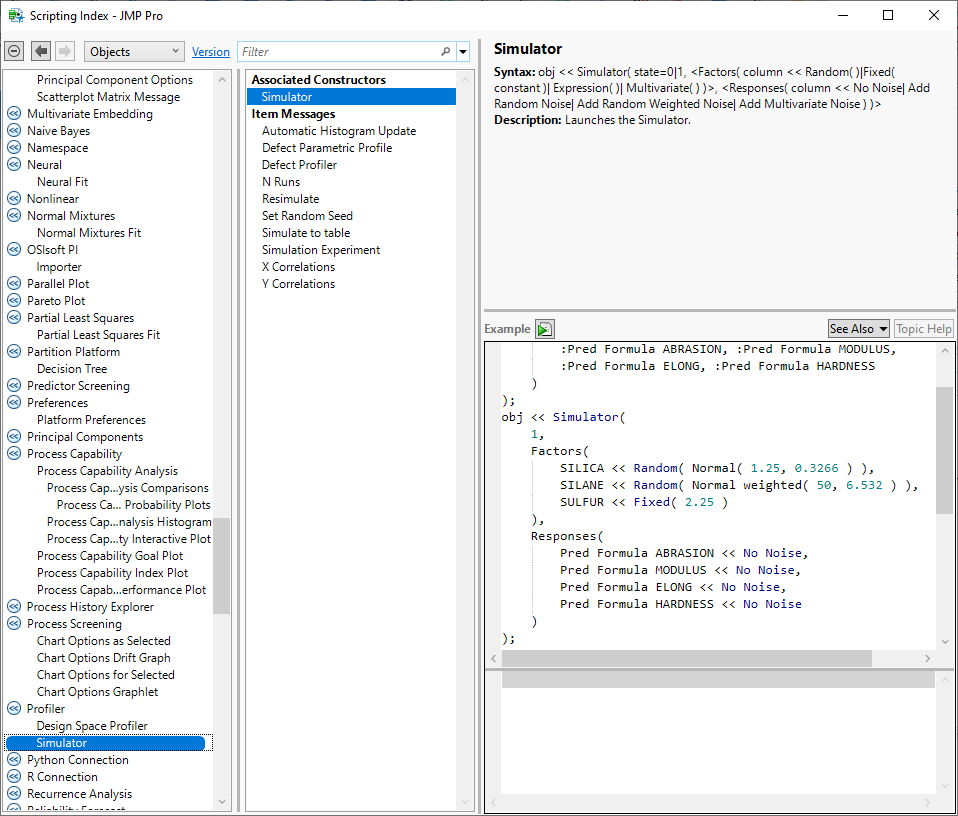
Yes, you can script the Profiler and the Simulator it provides. See Help > Scripting Index > Objects > Profiler and Simulator.
- Mark as New
- Bookmark
- Subscribe
- Mute
- Subscribe to RSS Feed
- Get Direct Link
- Report Inappropriate Content
Re: How to use JSL to find X variable range to meet spec limit by fixing other variables in Prediction Profiler?
@Mark_Bailey I finished the simulation for parameters, and collect all the simulation results already. Super cool!!! Thank you so much for your help.
The only challenge for me is to get the term value from the model script. What I used is to search "{Profiler(" and then "Term Value" to get all the terms into a list, and then simulate. The term value has numeric and character, some with "xxxx"n, some not, it's pretty difficult to make code for all different cases. Do you have easy way to get the Term value from the DoE model?
- Mark as New
- Bookmark
- Subscribe
- Mute
- Subscribe to RSS Feed
- Get Direct Link
- Report Inappropriate Content
Re: How to use JSL to find X variable range to meet spec limit by fixing other variables in Prediction Profiler?
By "get the term value from the model script," do you mean the parameter estimate in the Model table script? Did you save a table script for the model?
Character strings can be used for names. Some characters are disallowed in names. Use of improper names require a work-around.
Recommended Articles
- © 2026 JMP Statistical Discovery LLC. All Rights Reserved.
- Terms of Use
- Privacy Statement
- Contact Us


