How to run Monte Carlo for variation in Factors - Simulation Experiment/Stochastic Optimization

[#1]

Hello,

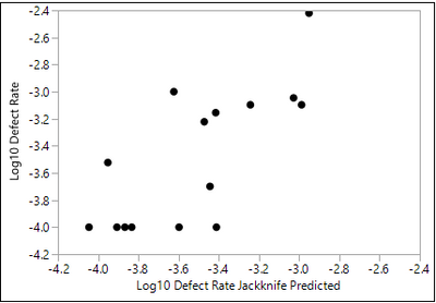
I am trying to understand how to utilize the "Simulation Experiment" under the Simulator red triangle to assess how my response is affected by random variation/distribution in my X factors, but am not sure how to interpret the results. It generates a separate "Gaussian Process Model of Log10 Defect Rate":

zjuv007_0-1589129599221.png

zjuv007_1-1589129615592.png

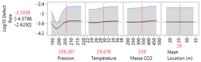
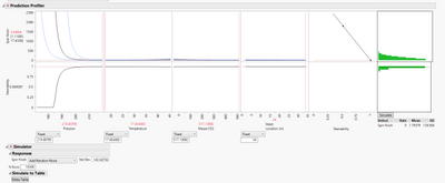
Below are my X factors in a fixed state currently:

zjuv007_2-1589130044772.png

I have a few questions:

1. Does the initial Desirability minimize only perform minimization on the prediction expression/equation generated, and not take into account random normal variation of the X factors?

2. When I run the Simulation Experiment, what is the Gaussian Process telling me? I want to generate a capability analysis of the Response due to random variation of my X factors... this doesn't appear to provide that information (I don't know how to interpret the Log10 Defect Rate)

3. Are there any resources/examples of this type of problem available somewhere I could reference?

[#2]

I have some questions and comments, and then I will try to answer your questions based on the information that you already provided.

1. What is your response?
2. What kind of model are you using?
3. Are the factors significant?
4. What effects are you modeling?

Here are my answers:

1. Yes, the desirability function represents the mean response because that is what the model represents. You could model the variance of the response as well and define its desirability separately.
2. There is a control in the Table outline to save the simulation results in a new data table for capability analysis.
3. What resources have you used so far? Have you read Help > JMP Documentation Library > Profilers guide?

[#3]

What is your response? My response is a manufacturing process of an amount of residual oil on a material, in PPM
What kind of model are you using? I am currently using a quadratic model with two way interactions
Are the factors significant? The quadratic terms are not of significance, leading to a more simply two way interaction and the linear terms (which are significant)
What effects are you modeling? The amount of residual oil depends upon the temperature, pressure, and amount of Co2 used in the chamber it is placed within. I was attempting to go beyond the normal prediction equation and into Stochastic Optimization, wherein it is my understanding that this will allow me to do additional experimental runs to represent the variation and unpredictability of my effect variables.

I have utilized the example of stochastic optimization: https://www.jmp.com/support/help/en/15.1/index.shtml#page/jmp/example-of-stochastic-optimization.sht...

When I don't necessarily know with full certainty that my effect factors can be controlled or will be an exact number, would the stochastic optimization provide assistance with this uncertainty?

[#4 · Accepted solution]

Thank you for the reference. Now I understand better what you are doing.

The simulation step after the optimization step assesses your current setting for each factor with the expected variation. It simulates future runs given the definition for each factor and the response. It is just about capability and defects. That information might be enough for your purpose.

The next step, Simulation Experiment, is not required but offers more information. This step uses your fitted model, not your experimental data. It uses a space-filling design for a computer experiment within the original factor space. A data table is created with the design and the estimated overall defect rate based on the simulated response for each run. It uses a Gaussian Process model with the defect rate from the computer experiment as an interpolator to predict and visualize the results of the experiment. Defect rates can vary by several orders of magnitude, so the rate is transformed with the log, base 10, function for stability.

How you define the random component of your factors in the Simulate feature will help you assess the effect of how well you can control them on the process.

[#5]

Thank you for this!

It is my understanding that the simulation experiment is beneficial in minimizing defect rate, as your optimization performed in the Simulation step after optimization may not provide the lowest yield. Is that an accurate assessment at a high level?

[#6]

You are correct!

[#7]

Just some other thoughts:

1. I don't understand what you mean by amount of oil in PPM.  Can't you measure the actual amount of residual oil (e.g., volume, weight, concentration, etc.).  The more continuous your measurement, the more efficient your study (and the less you need to rely on transformations)

2. Why would you simulate variation in the x's?  Why not study the variation in the x's?  Monte Carlo is more effective if you know the distribution, variation and consistency of the variation in the x's.  It seems to me you need some knowledge of the variation in the x's before you choose levels for your experiment.  If the random variation at one level overlaps the random variation at another level, it could be difficult to assign the variation.

[#8]

A great question.
This is an industry DOE which has already been run and am utilizing what data I have to inform. To my understanding, the oil is removed via supercitical CO2 chamber and the extract is measured via NMR spectro, converted to a PPM (I'm not fully detailed in the breakdown of that data at this current point).

To your second point, since the DoE study was already completed, I would hope to gain an understanding that the variation in our X's due to randomness could potentially have on our response and the capability. If, for example, the temperature variation is not well understood or is thought to be random within a specific range (e.g. 35 - 45 C), and only the low, mid, high were tested from the DoE,

I would still ask: what does the simulation experiment gain me in further understanding this system? Or is the Simulate of the x's good enough to study the variation in x's and their effect on the response?

[#9]

Sorry, I didn't realize you were working with an existing experimental data set that you didn't create.

Regarding your situational examples; The level setting in the experiment and the associated noise that changes during the experiment creates the inference or design space. In your hypothetical, "the temperature variation is not well understood", if the temp is not well understood, study it! How confident would you be in results from a simulation that assumes some distribution and some amount of total variation?, Or "is thought to be random within a specific range (e.g. 35 - 45 C), and only the low, mid, high were tested from the DoE", I would suggest that if the low were 35º and the high was 45º and a third level at the center 40º then you have a fairly good understanding of that space.  Realize, that a simulation is based on an algorithm (model) already known.  Perhaps the model was created as a result of an experiment.  The inference space of the experiment is still a restriction on the viability of the model.  Can you hypothesize what might happen as you use your model to predict outside of the inference space?  Of course, but you would be better served to actually run experiments over a wider inference space.