How to reconcile prediction profiler confidence intervals with parameter estimates for mixture design

[#1]

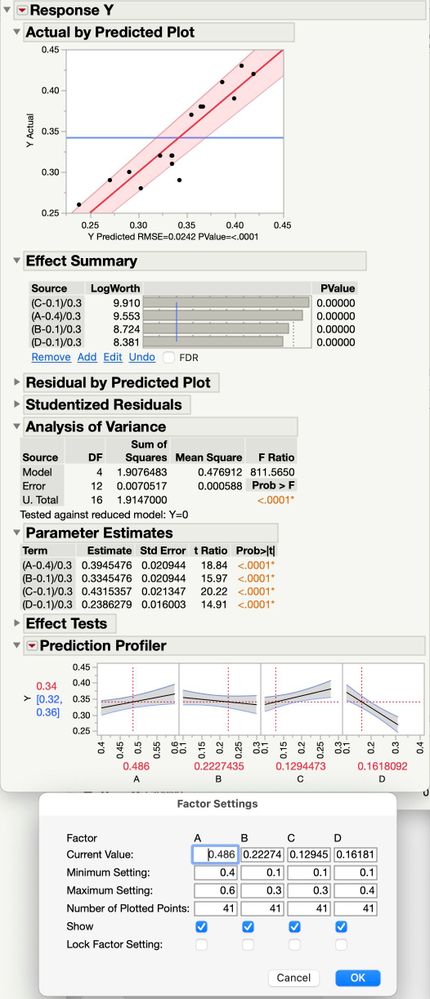
I have an mixture experiment with four components.  It's a custom design of 16 runs with no replication that started with a model that included interactions of two factors and three components.  The mixture constraint is that the four components sum to 1.0. The reduced model from the data has only the four main effects as statistically significant (p<.0001).

The prediction profiler plots show 95% confidence intervals that imply the "slope" of the effect of some significant factors could be zero; the gray band encompasses a horizontal line.  It also shows the factor having the smallest effect has the largest slope.

The profiler also shows the slope of the effect of component A changing as I change the amount of component C, even though there are no interactions in the model.  A has a slope of 0.05 units when C is at 0.1 and it has a slope of 0.02 units when C is 0.2.  Of course the amounts of the other components change to stay within the inference space, but why the change in slope?

The attached graphic shows what I'm seeing.  It also shows a Factor Settings dialog that has the min and max settings that were used in the mixture experiment.

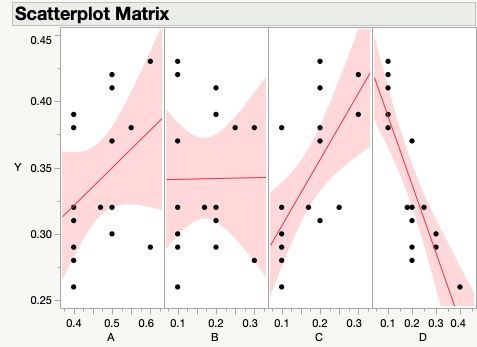
The scatterplots and the prediction profiler plots looks similar, they make it look like factor B is insignificant.  But if I leave B out of the model, the residual errors show that to be a mistake.

How do I interpret the slope and confidence intervals on the prediction profiler for this situation?  Or maybe how do I relate the parameter estimates to the prediction profiler?

[#2]

Just a further note when analyzing mixture designs...I would suggest using the Mixture Response Surface and Mixture Profiler rather than Prediction Profiler.  This will give you contour maps of the area created by the mixture of the components.  This can be easier to interpret.