- New to JMP? Let the Data Analysis Director guide you through selecting an analysis task, an analysis goal, and a data type. Available now in the JMP Marketplace!
- See how to install JMP Marketplace extensions to customize and enhance JMP.
- Subscribe to RSS Feed
- Mark Topic as New
- Mark Topic as Read
- Float this Topic for Current User
- Bookmark
- Subscribe
- Mute
- Printer Friendly Page
Discussions
Solve problems, and share tips and tricks with other JMP users.- JMP User Community
- :
- Discussions
- :
- Re: Different slopes between lin. regression and main axis of density elipse: wh...
- Mark as New
- Bookmark
- Subscribe
- Mute
- Subscribe to RSS Feed
- Get Direct Link
- Report Inappropriate Content
Different slopes between lin. regression and main axis of density elipse: why?
Hi JMP Community,
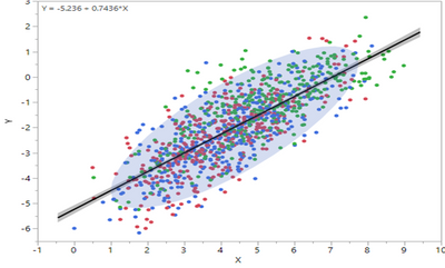
This may be a silly question but I cannot figure out why the slope of a linear regression does not match that of the main axis of the distribution elipse for the same data set (see below)?
Thanks for your help.
Sincerely,
TS
Accepted Solutions
- Mark as New
- Bookmark
- Subscribe
- Mute
- Subscribe to RSS Feed
- Get Direct Link
- Report Inappropriate Content
Re: Different slopes between lin. regression and main axis of density elipse: why?
Because the regression line assumes there is no error/variability in the X-values. All of the variability is in the Y. A density ellipse does not make that assumption. To see this, from your Fit Y by X plot, choose to Fit Orthogonal > Univariate Variances, Prin Comp. That line will be the major axis of the density ellipse.
- Mark as New
- Bookmark
- Subscribe
- Mute
- Subscribe to RSS Feed
- Get Direct Link
- Report Inappropriate Content
Re: Different slopes between lin. regression and main axis of density elipse: why?
Hi Dan
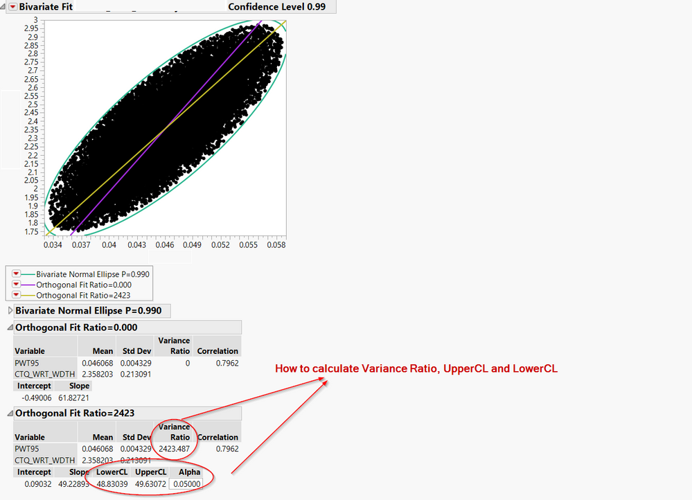
I have some question about Fit Orthogonal between Univariate Variances, Prin Comp and Fit X and Y.
From my understand. When we used Fit X and Y to plot Orthogonal line with no error. For Univariate Variances, Prin Comp It will add error variance ratio to calculatetion and finding the equetion symmetry between Upper and Lower Othogonal line.
My question is How Jmp can calculated variance ration, UpperCL and LowerCL ?. I still stuck this long time.
I very appreciate to you.
Thanks you
- Mark as New
- Bookmark
- Subscribe
- Mute
- Subscribe to RSS Feed
- Get Direct Link
- Report Inappropriate Content
Re: Different slopes between lin. regression and main axis of density elipse: why?
You could start with Help > Books > Basic Analysis > Bivariate. The Statistical Details at the end of this chapter provides this explanation:
Fit Orthogonal
Standard least square fitting assumes that the X variable is fixed and the Y variable is a
function of X plus error. If there is random variation in the measurement of X, you should fit a
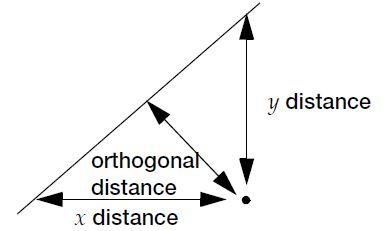
line that minimizes the sum of the squared perpendicular differences (Figure 5.26). However,
the perpendicular distance depends on how X and Y are scaled, and the scaling for the
perpendicular is reserved as a statistical issue, not a graphical one.
Figure 5.26 Line Perpendicular to the Line of Fit
The fit requires that you specify the ratio of the variance of the error in Y to the error in X. This
is the variance of the error, not the variance of the sample points, so you must choose carefully.
The ratio is infinite in standard least squares because is zero. If you do an
orthogonal fit with a large error ratio, the fitted line approaches the standard least squares line
of fit. If you specify a ratio of zero, the fit is equivalent to the regression of X on Y, instead of Y
on X.
The most common use of this technique is in comparing two measurement systems that both
have errors in measuring the same value. Thus, the Y response error and the X measurement
error are both the same type of measurement error. Where do you get the measurement error
variances? You cannot get them from bivariate data because you cannot tell which
measurement system produces what proportion of the error. So, you either must blindly
assume some ratio like 1, or you must rely on separate repeated measurements of the same
unit by the two measurement systems.
An advantage to this approach is that the computations give you predicted values for both Y
and X; the predicted values are the point on the line that is closest to the data point, where
closeness is relative to the variance ratio.
Confidence limits are calculated as described in Tan and Iglewicz (1999).
- Mark as New
- Bookmark
- Subscribe
- Mute
- Subscribe to RSS Feed
- Get Direct Link
- Report Inappropriate Content
Re: Different slopes between lin. regression and main axis of density elipse: why?
Hi Mark,
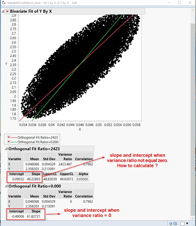
Thanks you for you comment. After i try to understand a concept of Fit Orthogonal with variance ration. From Jmp Document, I already knows concept and how to calculate a Intercept , Slope and variance ratio when variance ratio = 0.
Anyway, Jmp Document still not mention a theory of How to calculate a slope and intercept when variance ration not equal 0. Do you have any knowleadge about this ?
- Mark as New
- Bookmark
- Subscribe
- Mute
- Subscribe to RSS Feed
- Get Direct Link
- Report Inappropriate Content
Re: Different slopes between lin. regression and main axis of density elipse: why?
See this article for background on the computation of the orthogonal regression estimates.
Recommended Articles
- © 2026 JMP Statistical Discovery LLC. All Rights Reserved.
- Terms of Use
- Privacy Statement
- Contact Us


