- Subscribe to RSS Feed
- Mark Topic as New
- Mark Topic as Read
- Float this Topic for Current User
- Bookmark
- Subscribe
- Mute
- Printer Friendly Page
Discussions
Solve problems, and share tips and tricks with other JMP users.- JMP User Community
- :
- Discussions
- :
- Difference between JMP and Excel in dummy variable regression outputs
- Mark as New
- Bookmark
- Subscribe
- Mute
- Subscribe to RSS Feed
- Get Direct Link
- Report Inappropriate Content
Difference between JMP and Excel in dummy variable regression outputs
Hi all,
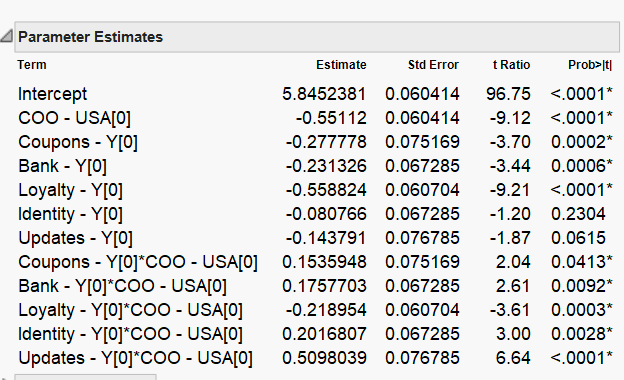
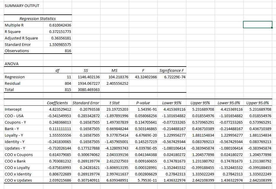
Newbie question here: I'm doing dummy variable regression using JMP for a school project. When I cross-referenced to Excel's version, I realized the coefficients are completely different even though the t-stats are the same.
JMP:
These two images are of JMP and as you can see as compared to the Excel's version, the figures are different even though I'm using the same attributes.
And it's not because of the interaction effect as I did with just the variables, without the interaction effect (e.g. COO x Coupons) and the results are still different.
Strangely, Excel's version seems more correct than the JMP's version, aligning more closely with my secondary and other primary research.
Any advice?
Accepted Solutions
- Mark as New
- Bookmark
- Subscribe
- Mute
- Subscribe to RSS Feed
- Get Direct Link
- Report Inappropriate Content
Re: Difference between JMP and Excel in dummy variable regression outputs
Excel is not more correct. They are just different. It has to do with the parameterization of the linear model. The choice is mathematically arbitrary but each way has its advantages. JMP uses effect parameterization. That way is supposed to make the parameter estimates more interpretable. They sum to zero, so the intercept is the mean response at the origin. The parameter for a given level is the change from the intercept. So an estimate of -0.55112 for COO - USA = 0 means that the mean for that level is 5.8482381 - 0.55112 = 5.2941181. The plots are meant to help interpret the selected model.
Since you are using numeric values with the correct nominal modeling type, JMP is correctly estimating the effect of these categorical predictors. The numeric code, though, might be interpreted by Excel as a continuous variable, since it has nothing like modeling type that is fundamental to statistical modeling and testing. That model could lead to a very different estimate, test, and interpretation.
See Help > Books > Fitting Linear Models > Appendix A: Statistical Details > The Factor Models.
- Mark as New
- Bookmark
- Subscribe
- Mute
- Subscribe to RSS Feed
- Get Direct Link
- Report Inappropriate Content
Re: Difference between JMP and Excel in dummy variable regression outputs
Hi Mark,
Thanks for the quick reply. I think that's exceedingly helpful.
Just want to take this chance to ask too: Do the negative estimates mean that the presence of those variables reduces preference (assuming preference is the LHS variable and it is coded as low = not preferred and high = preferred), relative to the baseline?
This will be an odd discovery as compared to Excel as those variables are expected to increase preference.
- Mark as New
- Bookmark
- Subscribe
- Mute
- Subscribe to RSS Feed
- Get Direct Link
- Report Inappropriate Content
Re: Difference between JMP and Excel in dummy variable regression outputs
The parameter is interpreted as the change in the response from the mean. A negative value does, in fact, indicate a drop in the response variable.
- Mark as New
- Bookmark
- Subscribe
- Mute
- Subscribe to RSS Feed
- Get Direct Link
- Report Inappropriate Content
Re: Difference between JMP and Excel in dummy variable regression outputs
Adding to the newbie question (pardon me), I'm also looking at the interaction between the different variables with the country of origin.
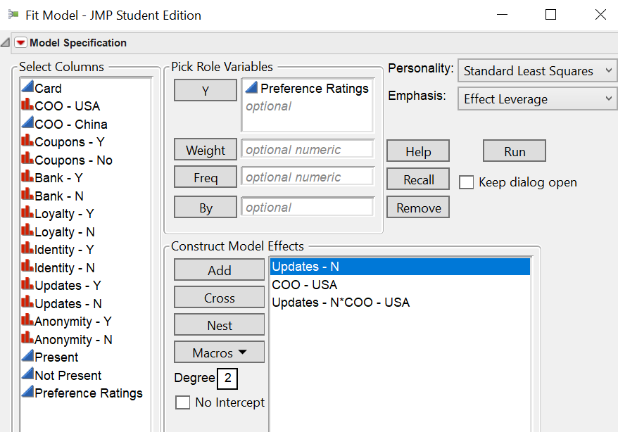
From a software's perspective, is this how we set up the model (Use the 'Cross' Button) to study interaction effect between Updates and COO - USA?
Thanks in advance, Mark.
Regards,
Fred
- Mark as New
- Bookmark
- Subscribe
- Mute
- Subscribe to RSS Feed
- Get Direct Link
- Report Inappropriate Content
Re: Difference between JMP and Excel in dummy variable regression outputs
Correct, select the data columns for the factors involved in the interaction and click Cross.
See the Macros button for many convenient shortcuts, such as Factorial to Degree. With degree set to 2, it will add all possible two-factors using the selected data columns.
- Mark as New
- Bookmark
- Subscribe
- Mute
- Subscribe to RSS Feed
- Get Direct Link
- Report Inappropriate Content
Re: Difference between JMP and Excel in dummy variable regression outputs
Hi Mark,
Thanks for your help once more. I appreciate your prompt reply and really help me better understand how to use JMP for my work.
I do have one last question: Is there an option for me to factor in clustered correlation. The issue is, my dummy variables are all treated as independent entries when some of them are done by the same respondent, which means I need to factor that in.
I understand other statistical software allows that through a unique variable, but is there a way I can do so with the Fit Model in JMP.
Thanks for your help.
Regards,
Fred
- Mark as New
- Bookmark
- Subscribe
- Mute
- Subscribe to RSS Feed
- Get Direct Link
- Report Inappropriate Content
Re: Difference between JMP and Excel in dummy variable regression outputs
I cannot picture your study and its data well enough to answer you latest question. (Note: I didn't say 'last' question.) What do you mean by 'factor in clustered correlation?' I know that it is related to 'dummy variables are all treated as independent entries' and 'done by the same respondent.'
A row in a JMP data table represents all the values that make up one observation. That is, you know the value of every variable (independent and dependent) for a complete record. Are you saying that there is another variable, Respondent, that identifies the observation, that respondents contribute more than one observation, and you want to account for Respondent variability in the response? If so, enter this variable in your data table and add it as a term in Fit Model. Be sure to select it, click the red triangle for Attributes, and select Random Effect.
- Mark as New
- Bookmark
- Subscribe
- Mute
- Subscribe to RSS Feed
- Get Direct Link
- Report Inappropriate Content
Re: Difference between JMP and Excel in dummy variable regression outputs
Hi Mark,
Thanks for the quick reply. Apologise that I wasn't specific enough in my explanation.
Yes you're right. A respondent contributes more than one observation, but the analysis interprets each observation as independent and as one respondent when the actual case it's not true.
What I want to do is to adjust for standard errors for such clustered correlation, in JMP's Fit Model.
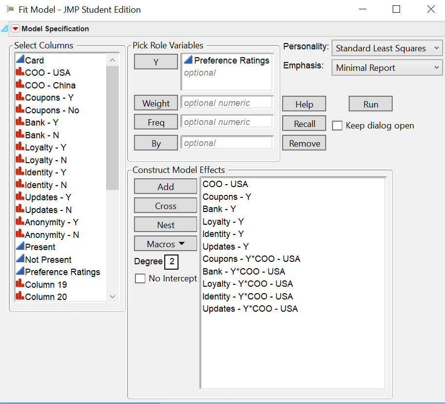
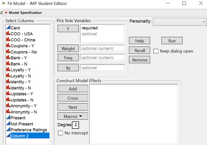
How can do I from the console below (if it's from here)? (:
Regards,
Fred
- Mark as New
- Bookmark
- Subscribe
- Mute
- Subscribe to RSS Feed
- Get Direct Link
- Report Inappropriate Content
Re: Difference between JMP and Excel in dummy variable regression outputs
First, as I said before, you don't need to create dummy variables in JMP. It is a statistical analysis and modeling software.
Second, create data columns as I described for the factors (not separate dummy variable columns for each factor level) so that each factor uses one data column and enter the value directly for each row.
Third, create a column (Respondent, for example) and populate it with values that identify the respondent for each row.
Now select Analyze > Fit Model. Select the response column and click Y. Select the factor columns and click Add or use Cross or a macro to add interaction effects to your model. Select the Respondent effect (not the data column), click the red triangle next to Attributes and select Random Effect. That change is all you have to do. You are simply distinguishing the type of effect of Respondent (random) from that of the other factors (fixed).
Recommended Articles
- © 2026 JMP Statistical Discovery LLC. All Rights Reserved.
- Terms of Use
- Privacy Statement
- Contact Us
