Simulating Multi-Step Processes and the Propagation of Error to the Final Response

[#1]

Imagine I have a multi-step process, like maybe an additive dispense process, where I'm using well characterized pumps to deliver set volumes to container and then at the end I check the mass of the container. What I would like to know is how much variation to expect in the final fill weight.  In my previous blog  I showed how to simulate one categorical level. To extend that approach to multiple inputs will be a little tricky, and take a lot more work. There is another way to approach the problem using several tools in JMP together. 

Step 1.  Make a data table like this:

In this table there are JUST 2 ROWS!  The :Final column has a formula that sums the first 4 columns.  There is some special formatting too. I went into Column Info, and Properties and added a Sigma property (about 2/3's of the way down the properties drop down list). Since I'm using a similar well defined pump for each step, I set sigma at 0.25 ml. 

Run this bit of JSL to make the table:

dt=New Table( "Propagation of Error Profiler",
	Add Rows( 2 ),
	New Column( "Step 1", Set Property( "Sigma", 0.25 ), Set Values( [10, 12] )),
	New Column( "Step 2", Set Property( "Sigma", 0.25 ), Set Values( [4, 5] )),
	New Column( "Step 3", Set Property( "Sigma", 0.25 ), Set Values( [20, 22] )),
	New Column( "Step 4", Set Property( "Sigma", 0.25 ), Set Values( [10, 12] )),
	New Column( "Final",Formula( :Step 1 + :Step 2 + :Step 3 + :Step 4 ))
);

Step 2. Profile the Formula

From the Graph menu, choose Profiler.   Add the "Final" column to the dialog and click OK.

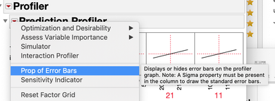
In the Profiler Red Triangle Menu (RTM) there is a special option available to help visualize the known error from the inputs. (i.e. its only there when sigma is speified as a column property.) Choose the Prop of Error Bars option.

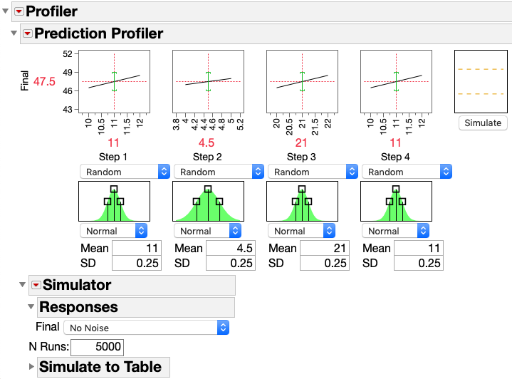
The next step in the profiler is to turn on the simulator. This option is under the Prediction Profiler outline bar RTM.  Since sigma is specified, the simulator automatically begins with the a normal distribution simulation of each variable at the mid point of the values specified in the table and the sigma in the column property.  (saves a lot of clicking around)

At this point your profiler should look like this:

Step 3 Start Simulating

Here is where it gets interesting.  I need to simulate running the process enough times that I can get good handle on how much the final weight will vary. To get a representative number of runs, change the 5000 in the N Runs to something like 500,000. (1 million is good to but 100 million will take a while, although the estimate at the end will be a little tiny bit better)

Then open the Simulate to Table outline bar and click the "make table" button.

Now I have a table with 500K runs. Each run is at a different random level for each of the process inputs.   Checking the distribution of the inputs and outputs I can see that the high side of my Final fill weight comes mostly from run where the inputs where on the high side of their range.

Now that I have a pretty good idea of the variation in Final fill weight, I can use the a typical workflow in the distribution platform to calculate a reasonable range that I can expect fill weights to occupy.  

Step 4  Geting 4 sigma limits

So, yes, I could just calculate a 4 standard deviation range on a calculator almost as fast as I can do what I'm going do do next.  But this is a little better and way more cool.

Analyze>Distribution> pick the simulated Final column. 

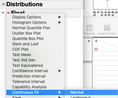
From the Distribution outline bar, pick Fit Continuous and pick Normal.

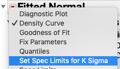
From the Fitted Normal outline bar, click on Set Spec Limits for k Sigma.

In this case, I'm going to pick 4 sigma. I want a Final fill weight that is extremely unlikely to occur to trigger an alarm or control action.

Last step, under the Fitted Normal outline bar, choose the option "Save Spec Limits"

and don't close this report.   (ideally JMP would dynamically make the spec limit property available to the profiler's simulator but this is not the case and we will have to manually transfer the values.)

Step 5

Technically I'm done. I did a massive Monte Carlo simulation of the effect of the process inputs on my Final fill weight and then estimated a set of limits that are unlikely to occur by happenstance. 

But wait, there's more.

I'm going to go back to the profiler report.  At the bottom, under the Simulator outline bar, turn on two options. 1. Spec Limits, and 2. Automatic Histogram Update.

In the spec limits dialog use 45.5 and 49.5 as the LCL and UCL. These are the rounded values we derived from the analysis in the distribution platfom.  

Next, at the top right of the profiler, there is a Simulate button next to the profiler graphs, click that.   Also try moving the sliders for the process inputs, by doing this I can see how much tolerance the process has for drift in one of more pumps.  I can also fairly redily see that if I had higher precision pumps I could tolerate a lot more dirft or calibration error without risking high or low Final fill weights. 

This is the script to generate the profiler in the figures

dt<<Profiler(
	Y( :Final ),
	Profiler(
		1,
		Prop of Error Bars( 1 ),
		Final << Response Limits(
			{Lower( 45.497, 0.0183 ), Middle( 47.500055, 1 ),
			Upper( 49.50311, 0.0183 ), Goal( "Match Target" ), Importance( 1 )}
		),
		Term Value(
			Step 1( 11, Lock( 0 ), Show( 1 ) ),
			Step 2( 4.5, Lock( 0 ), Show( 1 ) ),
			Step 3( 21, Lock( 0 ), Show( 1 ) ),
			Step 4( 11, Lock( 0 ), Show( 1 ) )
		),
		Simulator(
			1,
			Factors(
				Step 1 << Random( Normal( 11, 0.25 ) ),
				Step 2 << Random( Normal( 4.5, 0.25 ) ),
				Step 3 << Random( Normal( 21, 0.25 ) ),
				Step 4 << Random( Normal( 11, 0.25 ) )
			),
			Responses( Final << No Noise ),
			Automatic Histogram Update( 1 ),
			N Runs( 500000 ),
			Resimulate
		)
	),
	SendToReport(
		Dispatch(
			{"Prediction Profiler"},
			"Profile Simulator Histogram",
			FrameBox,
			{DispatchSeg(
				Hist Seg( 1 ),
				{Line Color( {65, 104, 68} ), Fill Color( "Green" ),
				Bin Span( 2, 0 )}
			)}
		),
		Dispatch(
			{"Prediction Profiler", "Simulator"},
			"Simulate to Table",
			OutlineBox,
			{Close( 0 )}
		),
		Dispatch(
			{"Prediction Profiler", "Simulator"},
			"Spec Limits",
			OutlineBox,
			{SetHorizontal( 1 )}
		)
	)
)

This script will generate the analysis from the distribution platform

dt<<Distribution(
	Continuous Distribution(
		Column( :Final ),
		Horizontal Layout( 1 ),
		Vertical( 0 ),
		Outlier Box Plot( 0 ),
		Capability Analysis( 0 ),
		Fit Distribution(
			Normal(
				Quantiles( 0.00003167124183312, 0.999968328758167, 0 ),
				Spec Limits( LSL( 45.500867399142 ), USL( 49.50097767193 ) )
			)
		),
		Customize Summary Statistics( N Missing( 1 ), N Unique( 1 ) )
	),
	SendToReport(
		Dispatch(
			{"Final"},
			"Distrib Histogram",
			FrameBox,
			{Frame Size( 372, 234 )}
		),
		Dispatch(
			{"Final"},
			"Quantiles",
			OutlineBox,
			{Close( 1 ), OutlineCloseOrientation( "Vertical" )}
		),
		Dispatch(
			{"Final"},
			"Summary Statistics",
			OutlineBox,
			{Close( 1 ), OutlineCloseOrientation( "Vertical" )}
		)
	)
)

I hope you find this useful.  I'm sure someone (or me) has written up this workflow before, but I couldn't it earlier this week, so here it is again.

Cheers,

B