- New to JMP? Let the Data Analysis Director guide you through selecting an analysis task, an analysis goal, and a data type. Available now in the JMP Marketplace!
- See how to install JMP Marketplace extensions to customize and enhance JMP.
Byron Wingerd's Blog
- JMP User Community
- :
- Blogs
- :
- Byron Wingerd
- :
- It's not Normal, or is it?
- Subscribe to RSS Feed
- Mark as New
- Mark as Read
- Bookmark
- Subscribe
- Printer Friendly Page
- Report Inappropriate Content
It's not Normal, or is it?
In several recent discussions about using parametric tests the question of whether the data is normally distributed (or passes a goodness of fit test for normality) has come up. In each of the cases the sample size was relatively low (<30) and the conclusion was that the data did not come from a normally distributed population. The next steps involved some convoluted transformation steps that overly complicated the analysis.
I started to wonder what the chances are of failing a goodness of fit test when the underlying population was actually normally distributed, or what's the type I error rate. On the other hand if the population was just a little skewed, nonnormal, how often would it pass a goodness of fit test?
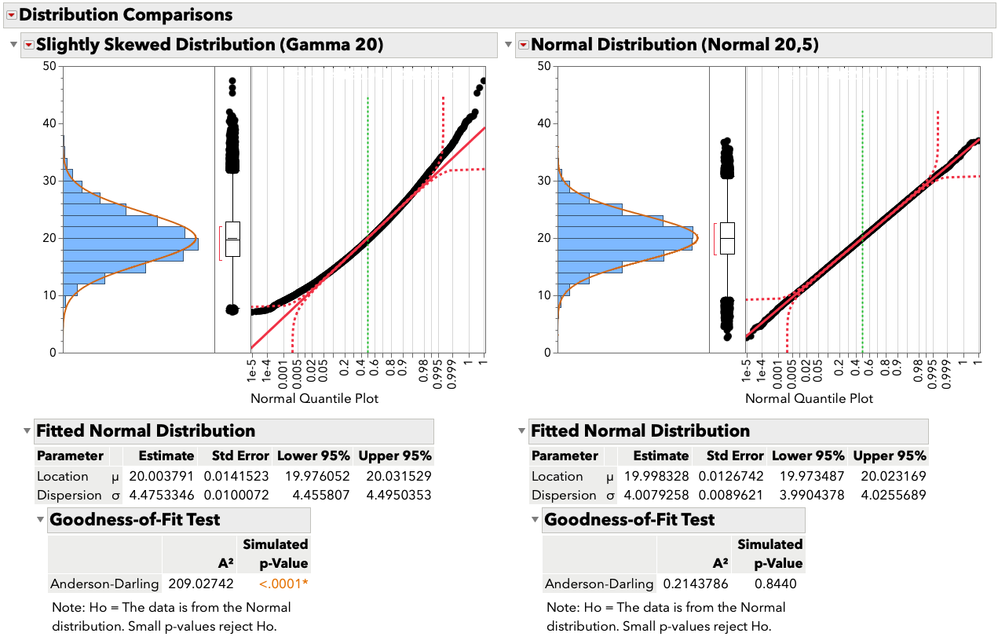
To start with I generated sets of 10 samples from normally distributed population and from a gamma distributed population using some random functions as formulas in a data table. Random normal (20,4) and Random Gamma(20). The population statistics clearly show that the normal distribution is normal and the gamma distribution fails a normality test (figure 1).
Figure 1. Distribution comparisons of populations from a normal or gamma distribution. Sample size is 10,000. With a large sample size the tails of the gamma distributed population (left panel) clearly fall outside the 95% confidence intervals (red dashed lines) of the normal probability regression line in the normal quantile plot.
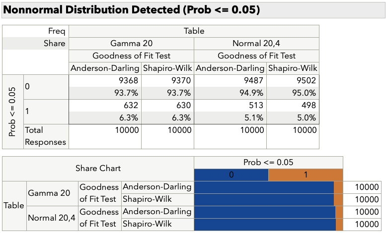
The a large data sets (n=100,000) was divided into groups of 10 and each subgroup (n=10,000) was tested for normality using the same tests used for the data set in figure 1. Small probability values reject the null hypothesis that the data is from a normal distribution so a cut-off of 0.05 was used to determine whether the subgroup passed the goodness of fit test. The tabulated results are presented in figure 2. Both the Anderson-Darling and Shapiro-Wilk goodness of fit tests flagged a similar proportion of the sample groups. Groups from the normal population failed about 5% of the time and groups from the gamma distributed population passed about 94% (failed about 6%) of the time.
Figure 2. Proportion of Samples failing Goodnes of Fit Tests. Sample groups (n=10) with a probability of being from a normal distribution <= 0.05 are labeled "1" and passing groups are labeled "0".
I was a little surprised at the type 1 error rate for the samples from the normal distribution (maybe I shouldn't have been..) This means with a small sample size about 1 in 20 times, data from an underlying normally distributed population will fail a goodness of fit test. Samples from a slightly skewed population had a similar detection rate.
Obviously the problem is the small sample size? The next step was to perform the same test groups with increasingly large sample sizes. Certainly the false positive rate will decrease dramatically with a little larger sample. The next step was to test subgroups of 30, with little effect, followed by subgroups of 100, 300 and 1000. Now, just to keep things even I wanted n=10,000 for the number of subgroups; however, the tables started to get big and the analysis started to get slow so I stopped with the sample size of 1000. Mostly be cause I'm not that patient and the trend was becoming obvious. In my vein of science, a sample size of 3 was the minimum, 10 was a lot, and 30 was just getting silly. As it turns out the right number is probably a lot higher to really evaluate the goodness of fit reliably. Figure 3 includes the proportion of samples failing the goodness of fit tests for the sample sizes I used.
Figure 3. Proportion of Nonnormal Samples. The proportion of nonnormal samples for each sample size is plotted for both the Anderson-Darling and Shapiro-Wilk test. Samples were from a population with a normal distribution.
From the data and analysis in these simulations I'm more cautious about accepting the results of from a goodness fit test without carefully looking at the data. I would be extremely hesitant to add a goodness of fit statistic to acceptance criteria or an SOP for handling data. Running with stats blindly is almost a safe as running with scissors? I guess this begs the question of how to better assess the assumptions of normality for parametric tests. Perhaps that's a good subject for a future blog post.
If you would like to improve on the method I used for challenging the false positive rate of a normality test, or just want to try to reproduce my results, I've included the script I used to generate data below. In there script there are notes on where to change the values for the table size and sample size.
Names Default To Here( 1 );

dt = New Table( "Source Data",
	Add Rows( 10000 ), //Change row number when using larger sample sizes
	New Column( "Normal", Numeric, "Continuous", Format( "Best", 12 ), Formula( Random Normal( 20, 4 ) ) ),
	New Column( "Gamma", Numeric, "Continuous", Format( "Best", 12 ), Formula( Random Gamma( 20 ) ) ),
	//Change the number of times the group column repeats for larger or smaller sample sizes
	New Column( "group", Numeric, "Continuous", Format( "Best", 12 ), Formula( Sequence( 1, N Rows(), 1, 10 ) ) )
);

rpt = New Window( "Distribution",
	dt << Distribution(
		Continuous Distribution(
			Column( :Normal ),
			Quantiles( 0 ),
			Summary Statistics( 0 ),
			Process Capability( 0 ),
			Fit Normal( Goodness of Fit( 1 ) )
		),
		Continuous Distribution(
			Column( :Gamma ),
			Quantiles( 0 ),
			Summary Statistics( 0 ),
			Process Capability( 0 ),
			Fit Normal( Goodness of Fit( 1 ) )
		),
		By( :group )
	)
);
Wait( 0 );
//Get tables from the report
dt1 = rpt["Distributions", "group=1", "Normal", "Fitted Normal Distribution", "Goodness-of-Fit Test", Table Box( 1 )] << Make Combined Data Table;
dt1 << set name( "AD" );
dt2 = rpt["Distributions", "group=1", "Normal", "Fitted Normal Distribution", "Goodness-of-Fit Test", Table Box( 2 )] << Make Combined Data Table;
dt2 << set name( "SW" );
rpt << Close Window;

//table formatting
dt1 << New Formula Column( Operation( Category( "Row" ), "Row" ), Columns( :Table ) );
dt2 << New Formula Column( Operation( Category( "Row" ), "Row" ), Columns( :Table ) );
dt1:Column 1 << Set Name( "Goodness of Fit Test" );
dt2:Column 1 << Set Name( "Goodness of Fit Test" );
Column( dt1, 7 ) << Set Name( "Fit" );
Column( dt2, 7 ) << Set Name( "Fit" );
Column( dt1, 8 ) << Set Name( "Prob" );
Column( dt2, 8 ) << Set Name( "Prob" );
dt3 = dt1 << Concatenate( dt2, Output Table( "Goodness of Fit Tests" ) );

Close( dt, nosave );Close( dt1, nosave );Close( dt2, nosave );
sfsdff
You must be a registered user to add a comment. If you've already registered, sign in. Otherwise, register and sign in.
- © 2026 JMP Statistical Discovery LLC. All Rights Reserved.
- Terms of Use
- Privacy Statement
- Contact Us


