- New to JMP? Let the Data Analysis Director guide you through selecting an analysis task, an analysis goal, and a data type. Available now in the JMP Marketplace!
- See how to install JMP Marketplace extensions to customize and enhance JMP.
JMPer Cable
A technical blog for JMP users of all levels, full of how-to's, tips and tricks, and detailed information on JMP features- JMP User Community
- :
- Blogs
- :
- JMPer Cable
- :
- Estimation of a Limit of Detection
- Subscribe to RSS Feed
- Mark as New
- Mark as Read
- Bookmark
- Subscribe
- Printer Friendly Page
- Report Inappropriate Content
This article appears in JMPer Cable, Issue 30, Summer 2015.
by Di Michelson di.michelson, Senior Analytical Training Consultant, SAS
Mark Bailey wrote an excellent article in Issue 29 of the JMPer Cable, detailing how to use data below a limit of detection. What do you do when you need to estimate that threshold of measurement? Analytical chemistry provides information about the concentration of an element or molecule in a substance (an analyte). Measurements of concentration have a natural bound at zero. The measurement process itself is variable, and it contains noise. Thus, measurements of a sample with known zero quantity of an analyte will result in non-zero responses. This background noise can be estimated to give a limit of detection (LOD): the upper bound on the noise of a measurement system.
To estimate the detection limit of the measurement method, we would like to find the lowest level of concentration where the results become indistinguishable from a zero reading. This is the point at which we would start to see signals for zero concentrations. Different methods for finding the LOD exist in the literature. Industry standards, including SEMI C10 (Guide for Determination of Method Detection Limits), ISO:11843 (Capability of Detection), and the International Union of Pure and Applied Chemistry (IUPAC) Compendium of Analytical Nomenclature1, discuss methodologies for determining the detection limit. Most authors advise the use of the calibration curve to fit a linear model, followed by inverse prediction to find the LOD.
We will examine various methods to fit a linear model to a calibration curve, followed by estimating a prediction interval for future observations at the zero level, and finally, using inverse prediction of the upper bound to estimate the LOD. We will consider ordinary least squares (OLS) regression to fit a linear model to the calibration curve. Other methods popular in the literature are based on weighting schemes.
A 100(1–α)% prediction interval is a range of values of a variable with the property that if many such intervals are calculated for several samples, 100(1–α)% of them will contain one observation from a future realization of the process. A prediction interval is different from a confidence interval. A confidence interval gives limits in which we expect a population parameter, such as a mean or variance, to occur. A prediction interval gives limits in which we expect a future individual observation to occur.
You can find formulas for prediction interval calculations in the literature. The formula depends on the number of future observations to
be predicted. See Ramirez2 for an accessible discussion of statistical intervals.
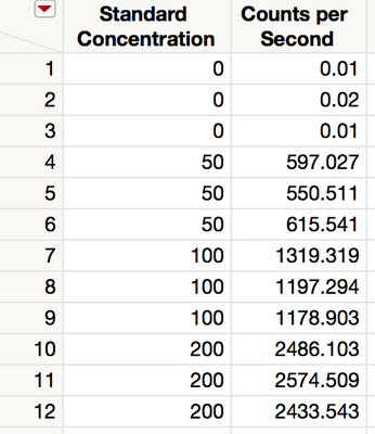
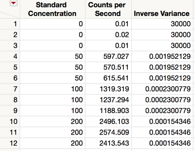
As an example, consider an inductively coupled plasma-mass spectrometry (ICP-MS) system that performs trace element analysis for the purpose of determining the amount of contaminants in a sample. A sample containing a known amount of a contaminant is measured. The response is signal intensity, measured in counts per second (CPS). The experiment is repeated for four known levels, including no contaminant at all. Figure 1 shows the data.
Figure 1 Data for contaminant levels and responses
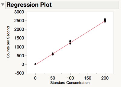
Figure 2 shows a graph of the measured values against the known values shows that the data seem to follow a linear trend. It is notable that the variability at the zero concentration level is much less than that at other levels.
Figure 2 Regression plot of measured values versus known values
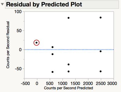
It can be hard to see the difference in variability at the zero level by using a scatterplot of the data. Instead, examine a plot of the residuals by the predicted response. The residual plot in Figure 3 clearly shows the variance is much higher where the element exists than where it doesn’t. There are three observations plotted in the red circle.
Figure 3 Plot of residuals versus the predicted response
Many physical characteristics show heteroscedasticity, or the variance of the response changing over the range of the data. The variability of physical data often increases as the response increases. Ordinary least squares regression makes the assumption of homoscedasticity, or equal variances across the range of data. Therefore, naively, it might make sense to pursue methods to stabilize the variance.
One method of variance stabilization is to use weighted least squares (WLS) regression, which weights the data by the reciprocal of the variance within each group. Most calibration problems do not use samples that are large enough to estimate group variances with low uncertainty. Therefore, another popular method is to model the variance as well as the mean. JMP implements this model using the Loglinear Variance personality of Fit Model. We will demonstrate OLS and these two methods of WLS regression.
Heteroscedasticity does not affect the bias of the regression coefficients (slope and intercept) using ordinary least squares. It does affect the standard errors of the regression coefficients. However, for typical data like our simulated data, the variance of the CPS for the blank is much less than that for the non-blanks, and the variance of the non-blanks is what we would like to use to find prediction intervals for the detection limit. The reason for this seeming contradiction is that using the variance of the CPS
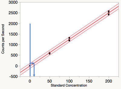
for the blank leads to prediction intervals that are too narrow. Narrow prediction intervals sound good but in practice can lead to unreasonable expectations. Therefore, the recommendation is to use ordinary least squares regression to find the prediction interval, followed by inverse prediction of the upper prediction limit to the regression line as shown in Figure 4. The Loglinear Variance model will also be shown to give reasonable predictions.
Figure 4 Ordinary least squares regression
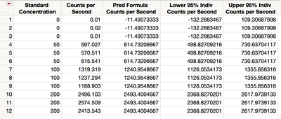
We use the Fit Least Squares platform from Fit Model to fit a line to the data. You save the prediction formula and prediction interval by selecting Save Columns > Prediction Formula and Save Columns > Individual Confidence Limit Formula from the red triangle next to Response Counts per Second. Figure 5 shows the data.
Figure 5 Data with saved prediction formula and intervals
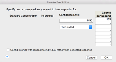
The estimate of the upper 95% prediction limit at zero is 109. Use inverse prediction to estimate the true concentration at this value. Return to the Fit Least Squares report. From the red triangle next to Response Counts per Second, select Estimates > Inverse Prediction. Enter 109 in the first blank space and click OK a shown in Figure 6.
Figure 6 Entering the estimated upper 95% prediction limit
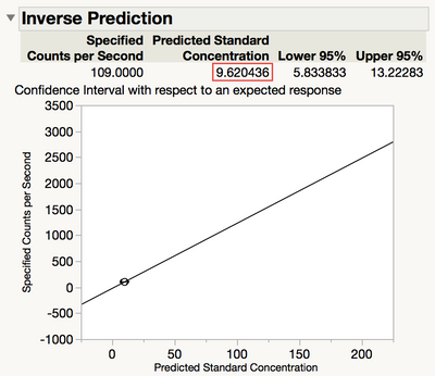
The predicted value of the response is 9.6, and that is our estimate of the detection limit as shown in Figure 7.
Figure 7 Predicted value of the response
Some industry standard documents, notably SEMI C10, recommend weighted least squares regression. Let’s compare the inverse prediction from the OLS prediction interval with that derived from WLS.
Weighted least squares uses weights on the data in order to stabilize the variance. An ad hoc method for weighting is to use the reciprocal variance of groups as the weights. To find the variance of each group, summarize the data using Tables > Summary. Add Standard Concentration as a grouping column, select Counts per Second, and then click Statistics > Variance to ask for the variance of CPS by group. Click OK.
Next, add a new column containing a formula to the summary table. This formula will contain the reciprocal of the variance of each group as shown in Figure 8.
Figure 8 Formula for the reciprocal of each group’s variance
The summary table contains the grouping variable, the sample size and variance for each group, and the inverse variance for each group as shown in Figure 9.
Figure 9 Summary table
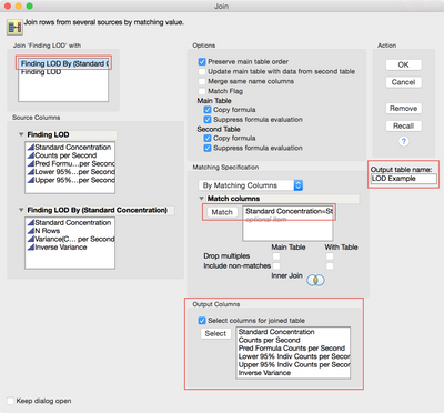
The inverse variance needs to go back into the original data table. Return to the original table and use Tables > Join to add the column of inverse variances as shown in Figure 10.
Figure 10 Joining the original and summarized data
The resulting table, shown in Figure 11, contains the columns from the original table in addition to the new weighting column.
Figure 11 Joined data
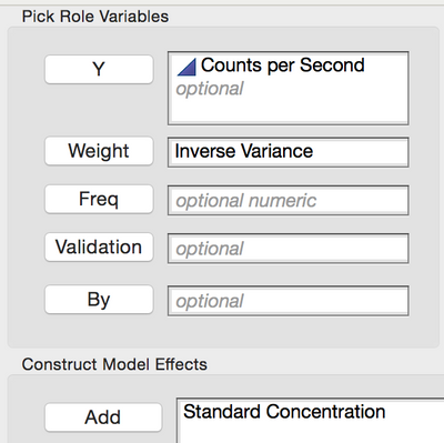
The regression model can now be fit again, this time using the Inverse Variance column in the Weight role as shown in Figure 12.
Figure 12 Specifying the Inverse Variance column
Again, save the prediction formula and prediction interval to the data table by clicking the red triangle and selecting Save Columns > Prediction Formula and Save Columns > Indiv Confidence Limit Formula. The OLS regression prediction columns have been hidden in the table shown in Figure 13.
Figure 13 Data with saved prediction formula and intervals
The estimate of the upper 95% prediction limit at zero is 0.03, four orders of magnitude smaller than that found by using OLS regression! Use inverse prediction once again to find the estimate of the detection limit. From the red triangle, select Estimates > Inverse Prediction. Enter 0.03 and click OK.
Figure 14 Inverse Prediction for Standard Concentration
As shown in Figure 14, the prediction is 0.0014, which is the estimate of the detection limit. This number is much smaller than that given by OLS regression (9.6). It may seem like a smaller number would be better, but WLS can lead to estimates that are known to be ridiculously small by the practitioner. For example, matching systems is sometimes done using the LOD. LODs that are too small can lead to systems that are not matched statistically, but for all practical purposes, can be considered to measure the same. This can lead to problems justifying the use of good systems with auditors.
One reason the prediction limit is so small, which results in a similarly small estimated detection limit, is that the group variance for the zero level is much less than the group variance for the other levels. Therefore, the inverse variance of the zero level is huge compared with the others.
One remedy for this is to model not only the mean response but the variance of the response as well. This method is particularly useful if you can assume the variance is proportional to the mean, for example. In addition to modeling the mean response with regressors, the Loglinear Variance model uses regressors to model the log of the variance. That is,
where the columns of X are the regressors for the mean response and the columns of Z are the regressors for the variance of the response. The parameters of the model for the mean are β, and the parameter of the model for the variance is λ. Find more information on the Loglinear Variance model in Fitting Linear Models from Help > Books in JMP.
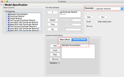
Using Fit Model, specify the Counts per Second as Y and Standard Concentration as the Mean Effect. Next, select the Loglinear Variance personality as shown in Figure 15. Select the Variance Effects tab at the bottom, add the Standard Concentration, and then run the model.
Figure 15 Fit Model Specification
The Loglinear Variance Fit report contains estimates of both β, and λ, , as well as fit statistics. Save the prediction formula and prediction interval by clicking the red triangle next to Loglinear Variance Fit and selecting Save Columns > Prediction Formula, then again, Save Columns > Indiv Confidence Interval. Figure 16 shows the prediction limits saved in the data table.
Figure 16 Upper prediction limit
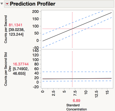
The upper prediction limit is 81. The Fit LogVariance report does not allow for inverse prediction, but it is simple to do with the Profiler. Return to the Fit LogVariance window. From the red triangle, select Profilers > Profiler. Drag the Standard Concentration slider to the left until the prediction of Counts per Second is near 81 (Figure 17). You can adjust the scale of the X axis if necessary to zoom in on the region of interest.
Figure 17 Inverse predictions in the Prediction Profiler
The inverse prediction is around 6.9, still a smaller number than 9.6 that was found using OLS regression, but much more reasonable than 0.0014 found using inverse variance weights.
Reasonable predictions are found in this example by both OLS regression and Loglinear Variance regression. In both models, the variance of the blanks does not overwhelm the calculation of the prediction interval for the zero level. The variance of the blanks leads to very small estimated detection limits when using the inverse variance as weights. Using OLS regression leads to a more conservative estimate of the detection limit as does Loglinear Variance regression. As George Box famously said, all models are wrong, but some models are useful. In the case of finding the limit of detection, OLS and Loglinear Variance regression models lead to useful inverse predictions.
References:
- Inczedy, J., Lengyel, T., & Ure, A.M. (1998). Compendium of Analytical Nomenclature, Third Edition. Available at http://old.iupac.org/publications/analytical_compendium/.
- Ramírez, José G. (2009). Statistical Intervals: Confidence, Prediction, Enclosure. Available at http://www.jmp.com/software/whitepapers/.
- © 2026 JMP Statistical Discovery LLC. All Rights Reserved.
- Terms of Use
- Privacy Statement
- Contact Us






You must be a registered user to add a comment. If you've already registered, sign in. Otherwise, register and sign in.