- New to JMP? Let the Data Analysis Director guide you through selecting an analysis task, an analysis goal, and a data type. Available now in the JMP Marketplace!
- See how to install JMP Marketplace extensions to customize and enhance JMP.
Uncharted
- JMP User Community
- :
- Blogs
- :
- Uncharted
- :
- Contour Plot Areas
- Subscribe to RSS Feed
- Mark as New
- Mark as Read
- Bookmark
- Subscribe
- Printer Friendly Page
- Report Inappropriate Content
Some of the following code probably needs JMP 15 for XML import support, at least. It is also using a deep understanding of the displaybox tree that will need adjustments in the future.
@datanaut asked
dt = Open( "$sample_data/big class.jmp", invisible );

magenta = RGB Color( 1, 0, 1 );// pure magenta

cp = dt << Contour Plot(
	X( :weight, :height ),
	Y( :age ),
	Show Boundary( 0 ),
	Show Data Points( 0 ),
	Fill Areas( 1 ),
	Label Contours( 0 ),
	Transform( "Range Normalized" ),
	Color Theme( "White to Black" ),
	Show Boundary( 0 ),
	Specify Contours( Min( 12.5 ), Max( 16.5 ), N( 9 ) ),
	SendToReport( Dispatch( {}, "Contour Plot Graph", FrameBox, {Frame Size( 623, 512 ), Background Color( magenta )} ) )
);

ymin = (Report( cp )[axisbox( 1 )] << getscript)["Min"];
ymax = (Report( cp )[axisbox( 1 )] << getscript)["Max"];
xmin = (Report( cp )[axisbox( 2 )] << getscript)["Min"];
xmax = (Report( cp )[axisbox( 2 )] << getscript)["Max"];
Show( xmin, xmax, ymin, ymax );

cp << minimizewindow( 1 );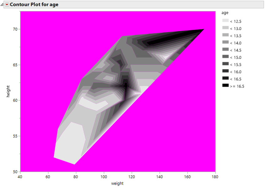
Path one was very short. I discovered contour plot has a message to <<saveContours. It makes a data table, but the contour descriptions don't make clean loops.
Path two was counting pixels, probably similar to @gzmorgan0 approach. It works, but has some flaws which you can see foreshadowed in the image above. I made the background that ugly magenta shade on purpose so I could easily hunt for gray pixels. But if you look closely, you can see some magenta leaking through between the regions. Bummer! Anti-aliasing at work! Normally, on a white background, you almost wouldn't notice, but the gray-scale transition between colors is still there.
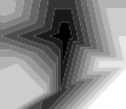
Anyway, the code below attempts to place the magenta-tinged pixels into a nearby gray area. Maybe it does a balanced job of making errors to either side. Without the magenta, it would all be shades of gray and the code would not be able to see a decision was needed. (This appears to run on JMP 14 and 15.)
pixels = (Report( cp )[framebox( 1 )] << getimage) << getpixels;
// trim non magenta edges. not sure why there are extra pixels...
For( ileft = 1, ileft < N Cols( pixels ), iLeft += 1,
	If( pixels[N Rows( pixels ) / 2, ileft] == magenta,
		Break()
	)
);
For( iright = N Cols( pixels ), iright > ileft, iright -= 1,
	If( pixels[N Rows( pixels ) / 2, iright] == magenta,
		Break()
	)
);
For( itop = 1, itop < N Rows( pixels ), itop += 1,
	If( pixels[itop, N Cols( pixels ) / 2] == magenta,
		Break()
	)
);
For( ibottom = N Rows( pixels ), ibottom > itop, ibottom -= 1,
	If( pixels[ibottom, N Cols( pixels ) / 2] == magenta,
		Break()
	)
);
If( ileft > 10 | itop > 10 | iright < N Cols( pixels ) - 10 | ibottom < N Rows( pixels ) - 10,
	Throw( "trimming error" )
);
pixels = pixels[itop :: ibottom, ileft :: iright];

colorCounts = [=> 0];

spiral = [-1 -1, -1 0, -1 1, 0 1, 1 1, 1 0, 1 -1, 0 -1, -2 -2, -2 -1, -2 0, -2 1, -2 2, -1 2, 0 2, 1 2, 2 2, 2 1, 2 0, 2 -1, 2 -2, 1 -2, 0 -2, -1 -2];

grays = [=> ];
For( i = 0, i <= 255, i += 1,
	grays[RGB Color( i / 255, i / 255, i / 255 )] = i
);
temp = pixels;
For( i = 1, i <= N Items( pixels ), i += 1,
	// pixels that are not magenta and not gray, but are antialiased values...
	// force them to the gray of a near pixel
	If( pixels[i] != magenta,
		{r, g, b} = Color To RGB( pixels[i] );
		If( (r != g & r == b),
			rowidx = Floor( (i - 1) / N Cols( pixels ) ) + 1; // nc is the number of columns in the 2D pixmat
			colidx = Mod( (i - 1), N Cols( pixels ) ) + 1; // rowlocs and collocs are 2D indexes (1-based)
			For( j = 1, j <= N Rows( spiral ), j += 1,
				// if this has an array out of bounds, make sure there is magenta pad all around
				color = pixels[rowidx + spiral[j, 1], colidx + spiral[j, 2]];
				If( grays << Contains( color ),
					temp[i] = color;
					Break();
				);
			);
		);
	);
	colorCounts[temp[i]] += 1;
);
pixels = temp;
totalpixels = Sum( colorCounts << getvalues );
If( totalpixels != N Rows( pixels ) * N Cols( pixels ),
	Throw( "error counting pixels" )
);

areaPerPixel = 1;//((ymax - ymin) * (xmax - xmin)) / totalpixels;

New Window( "Check polygons are inside the magenta area", New Image( pixels ) );
pixelcount = 0;
For( ii = 0, ii <= 255, ii += 1,
	i = ii / 255;
	If( colorcounts[RGB Color( i, i, i )] > 0,
		thisarea = colorcounts[RGB Color( i, i, i )] * areaPerPixel;
		Write( "\!ngray=", If( i == 0, "black", i == 1, "white", Char( i, 7, 3 ) ), " \!tarea=", Char( thisarea, 5 ) );
		pixelcount += colorcounts[RGB Color( i, i, i )];
		pixels[Loc( pixels == RGB Color( i, i, i ) )] = RGB Color( 0, 1, 0 );
	);
);
thisarea = colorcounts[magenta] * areaPerPixel;
Write( "\!nmagenta \!tarea=", Char( thisarea, 7, 3 ) );
pixelcount += colorcounts[magenta];
pixels[Loc( pixels == magenta )] = RGB Color( 0, 1, 0 );
New Window( "Check polygons are inside the magenta area", New Image( pixels ) );

Write( "\!nidentified \!tarea=", Char( pixelcount * areaPerPixel, 7, 3 ) );
Write( "\!nall graph \!tarea=", Char( totalpixels * areaPerPixel, 7, 3 ) );

Write( "\!noverlooked \!tarea=", Char( (totalpixels - pixelcount) * areaPerPixel, 7, 3 ) );
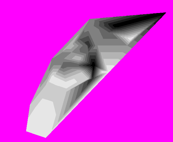
Here's the cleaned up image
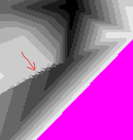
There is still some raggedness but it might be balanced out elsewhere:
The result is a table in the log window.
gray=black area=2598
gray=0.098 area=2973
gray=0.200 area=3781
gray=0.302 area=5003
gray=0.400 area=8528
gray=0.502 area=12535
gray=0.600 area=11081
gray=0.702 area=8382
gray=0.800 area=12718
gray=0.902 area=13074
magenta area=238302
identified area=318975
all graph area=318976
overlooked area=1.000
The overlooked pixel is a nearly pure magenta pixel at the top right corner. Didn't try to track it down further.
Path three is probably the best if you can make it work; it depends on JMP writing an SVG file in the same way, and may be dependent on this particular example as well. The answers are very similar to the second try, and should be more correct. (This depends on features in JMP 15.) Key to understanding the SVG path: column 3 of the matrix is negative for the end of a segment; the start/end arrays locate the segments in the path matrix.
(Report( cp )[framebox( 1 )]) << savepicture( "$temp/deletemeGraph.svg" );
(Report( cp )[framebox( 2 )]) << savepicture( "$temp/deletemeLegend.svg" );
Rename File( "$temp/deletemeGraph.svg", "deletemeGraph.xml" );
Rename File( "$temp/deletemeLegend.svg", "deletemeLegend.xml" );
dtSVGGraph = Open(
	"C:\Users\v1\AppData\Local\Temp\deletemeGraph.xml",
	XML Settings( Stack( 1 ), Row( "/svg/g/g/g/g/g/path/@d" ), Row( "/svg/g/g/g/g/path/@d" ),
		Col( "/svg/g/g/g/g/g/@fill", Column Name( "color" ), Fill( "Use Once" ), Type( "Character" ), Format( {"Best", 15} ), Modeling Type( "Continuous" ) ),
		Col( "/svg/g/g/g/g/g/path/@d", Column Name( "path" ), Fill( "Use Once" ), Type( "Character" ), Format( {"Best", 15} ), Modeling Type( "Continuous" ) ),
		Col( "/svg/@width", Column Name( "width" ), Fill( "Use Once" ), Type( "Table Variable" ), Format( {"Best", 15} ), Modeling Type( "Continuous" ) ),
		Col( "/svg/@height", Column Name( "height" ), Fill( "Use Once" ), Type( "Table Variable" ), Format( {"Best", 15} ), Modeling Type( "Continuous" ) ),
		Col( "/svg/g/@fill", Column Name( "colorAlternate" ), Fill( "-", "/svg/g" ), Type( "Character" ), Format( {"Best"} ), Modeling Type( "Continuous" ) ),
		Col( "/svg/g/g/g/g/path/@d", Column Name( "path" ), Fill( "Use Once" ), Type( "Character" ), Format( {"Best"} ), Modeling Type( "Continuous" ) ) ),
	XML Wizard( 0 )
);

For( i = 1, i <= N Rows( dtSVGGraph ), i += 1,
	If( dtSVGGraph:color[i] == "",
		dtSVGGraph:color[i] = dtSVGGraph:colorAlternate[i]
	)
);
dtSVGGraph << deletecolumns( {colorAlternate} );

dtSVGLegend = Open(
	"C:\Users\v1\AppData\Local\Temp\deletemeLegend.xml",
	XML Settings(
		Stack( 1 ),
		Row( "/svg/g/g/g/g/g/text" ),
		Row( "/svg/g/g/g/g/text" ),
		Col( "/svg/g/g/g/g/g/@fill", Column Name( "color" ), Fill( "Use Once" ), Type( "Character" ), Format( {"Best", 15} ), Modeling Type( "Continuous" ) ),
		Col( "/svg/g/g/g/g/g/text", Column Name( "text" ), Fill( "Use Once" ), Type( "Character" ), Format( {"Best", 15} ), Modeling Type( "Continuous" ) ),
		Col( "/svg/g/g/g/g/text", Column Name( "textAlternate" ), Fill( "Use Once" ), Type( "Character" ), Format( {"Best", 15} ), Modeling Type( "Continuous" ) ),
		Col( "/svg/g/g/g/g/g/rect/@y", Column Name( "y" ), Fill( "Use Once" ), Type( "Numeric" ), Format( {"Best", 15} ), Modeling Type( "Continuous" ) ),
		Col( "/svg/g/g/g/g/rect/@y", Column Name( "y" ), Fill( "Use Once" ), Type( "Numeric" ), Format( {"Best", 15} ), Modeling Type( "Continuous" ) ),
		Col( "/svg/g/@fill", Column Name( "colorAlternate" ), Fill( "-", "/svg/g" ), Type( "Character" ), Format( {"Best"} ), Modeling Type( "Continuous" ) ) ),
	XML Wizard( 0 )
);
dtSVGLegend << selectwhere( Is Missing( y ) );
dtSVGLegend << deleterows;
For( i = 1, i <= N Rows( dtSVGLegend ), i += 1,
	If( dtSVGLegend:color[i] == "",
		dtSVGLegend:color[i] = dtSVGLegend:colorAlternate[i]
	);
	If( dtSVGLegend:text[i] == "",
		dtSVGLegend:text[i] = dtSVGLegend:textAlternate[i]
	);
);
dtSVGLegend << deletecolumns( {textAlternate, y, colorAlternate} );
//dtSVGGraph<<sort(by(color),replacetable(1));
//dtSVGLegend<<sort(by(color),replacetable(1));
totalarea = 0;
Write( "\!n these are pixel counts for each color:" );
For( i = 1, i <= N Rows( dtSVGGraph ), i += 1,
	p = Char To Path( dtSVGGraph:path[i] );
	c = dtSVGGraph:color[i];
	If( dtSVGGraph:color[i] != dtSVGLegend:color[i],
		Throw( "color error" )
	);
	wide = Num( (dtSVGGraph << getproperty( "width" ))[1][1][1] );
	high = Num( (dtSVGGraph << getproperty( "height" ))[1][1][1] );
	//
	// p has many discontinuous areas, get the areas and sum them
	//
	ends = Loc( p[0, 3] < 0 );
	starts = 1 |/ (ends[1 :: N Rows( ends ) - 1] + 1);
	area = 0;
	For( isg = 1, isg <= N Items( ends ), isg += 1,
		xx = p[starts[isg] :: ends[isg], 1];
		yy = p[starts[isg] :: ends[isg], 2];
		area += Polygon Area( xx, yy );
	);
	Write( "\!n", c, " \!t", dtSVGLegend:text[i], " \!t", area );
	totalarea += area;
);
Write( "\!n------ total of gray pixels --------" );
Write( "\!n", "total \!t", " ", totalarea );
Write( "\!nTwo ways to represent the size of the graph's frame..." );
Write( "\!n", "frame \!t", " ", wide * high, " pixels" );
Write( "\!nThis is the product of the xaxis length * yaxis length:" );
Write( "\!n", "frame \!t", " ", (xmax - xmin) * (ymax - ymin), " data^2" );
Write( "\!nYou might use the frame's ratio of pixels to data^2 to convert the pixel counts for each color." );
Close( dtSVGGraph, nosave );
Close( dtSVGLegend, nosave );
The log output is reversed from last time...
these are pixel counts for each color:
#E6E6E6 < 12.5 13026.06075
#CCCCCC < 13.0 12648.7232
#B3B3B3 < 13.5 8322.47330000002
#999999 < 14.0 10780.35015
#808080 < 14.5 12529.58585
#666666 < 15.0 8507.05305
#4D4D4D < 15.5 4961.26459999998
#333333 < 16.0 3712.89360000002
#191919 < 16.5 2922.03675000001
#000000 >= 16.5 2535.49285
------ total of gray pixels --------
total 79945.9341
Two ways to represent the size of the graph's frame...
frame 318976 pixels
This is the product of the xaxis length * yaxis length:
frame 3150 data^2
You might use the frame's ratio of pixels to data^2 to convert the pixel counts for each color.
The pixel counts include decimals because they are computed as the areas of a bunch of small polygons that the SVG file uses to make the graph. Since SVG is variation of XML, I used the XML wizard to generate the XML Settings to read the two SVG files. One of the SVG files was saved from frame(1), the graph, and the other was saved from frame(2), the legend. The log output is labeled with the legend text, pulled from the SVG file. In JMP 15, the legend is in a second frame. That appears to be changing for JMP 16; if you carefully remove the legend related bits it still works, without the labels.
- © 2026 JMP Statistical Discovery LLC. All Rights Reserved.
- Terms of Use
- Privacy Statement
- Contact Us
You must be a registered user to add a comment. If you've already registered, sign in. Otherwise, register and sign in.