What is Acceptance Sampling?

[#1]

Acceptance Sampling

Acceptance sampling indicates whether an entire lot of product should be accepted or rejected. It enables both producers and consumers to test if a batch of products are acceptable, that is, do they meet specifications. With attributes one often thinks in terms of categorical responses, usually visual characteristics of the part.  You typically inspect for defects, such as discoloration, blemishes, tears, or scratches and record the number of defects or the number of defective components. As shown in the photograph above one could count the blemishes on the lemon and lime to determine how many defects were present.

However, it should be noted acceptance sampling does not improve the quality of the process in any way, and is never a substitute for good quality control processes. Refer to the Quality and Process learning library for details and examples of quality processes.  Acceptance sampling is useful as a decision-making tool for accepting or rejecting large scale manufactured goods and resources. In particular, in cases when the quality of a supplier's process is unknown, acceptance sampling may be a good option as opposed to 100% inspection.

Some reasons for acceptance sampling ( 2017, Acceptance Sampling in Quality Control 3rd Ed., Schilling, E.G, & Neubauer, D. V.)

1. Tests are destructive, therefore requiring sampling
2. Process not in control, involving sampling to evaluate the product
3. 100% sampling is inefficient, where as, 0% provides no assurance
4. Special causes might occur after process inspection ( after control chart is plotted )
5. Customers require sampling plans

Brief History

Coming out of Bell Laboratories in 1924 the science of acceptance sampling can be linked to some of the department members, including, H. F. Dodge, R. B. Miller, W. A. Shewhart and others. Other notables who became members of the department included, H. G. Romig. Notable because of the Dodge-Romig curves, Dodge-Romig tables that ones finds in the literature are attributed to the great minds of the department.  In 1925-1926, the terminology of acceptance sampling, including, operating characteristic curve, average total inspection, Type A and Type B risks and others is yet another example or direct result of the efforts of the Western Electric Bell Laboratories.  Distinction between acceptance sampling and acceptance quality control arose from military standards during World War II.  While the latter can be compared to process quality control the former advise a set of specific conditions for acceptance or rejection of a currently inspected lot.

In brief, quality process control is the aspect of the quality system. At the most basic level, or the simplest acceptance sampling plan can be noted as:

1. We inspect or test a single sample of a product lot.
2. If the sampled item is good, then one accepts the entire lot.
3. If the sampled item is defective, reject the entire lot.

So, we take one sample from the lot and then extrapolate from that sample to make an inference about whether the entire batch is acceptable.

Now that we understand why this is useful for safeguarding quality we can discuss an example. For example, you receive a shipment of 15,000 coffee mugs. With acceptance sampling, you develop a plan to determine how many coffee mugs you need to inspect (sample size) and how many defects are allowed within the sample (acceptance number). Inspecting and testing every coffee mug will take too much time and most likely cost too much money.  So as we noted above, it's much more efficient to examine only a few coffee mugs to determine whether the full shipment is ready to use, or if you should send the lot back to your supplier unless of course you are purchasing a mug made by skilled hands.

But how many should you look at? By using acceptance sampling, it can help you determine how many coffee mugs to examine, and how many defective coffee mugs you can permit and still accept the delivery of the shipment.

WHICH SHOULD I CHOOSE?

ACCEPTANCE SAMPLING BY ATTRIBUTES OR BY VARIABLES?

If you want to use acceptance sampling to evaluate a batch, lot or shipment of products, you first need to decide which method is best for your situation: acceptance sampling by attributes or by variables. 

Acceptance sampling by attributes assesses either the number of defects or the number of defective items in a sample. You might tally the total number of defects, in which case each defect in a single item with multiple defects is counted. Alternatively, you can count defective items, in which case the first problem makes an item defective, and you move on to evaluate the next item in your sample.

Attribute plans are generally easy to carry out: you randomly select a sample of n units from a collection ( lot ) of N units. Count the number of defectives. If there are fewer defectives than your acceptance number c, accept the lot. If there are more defectives than the acceptance number c, reject it. 

For example, suppose you're receiving 10,000 coffee mugs. You will inspect 28 of them. If there are 0, 1, or 2 defective coffee mugs, you can accept the delivery of the shipment.  But if the sample contains more than 2 defectives, you'll reject the lot.

Acceptance sampling by variables is based on quality characteristics you can measure. For example, you might measure the weight of the mugs, the length of the handles, the thickness of the mug. 

JMP SAMPLING PLANS

In JMP, you select Add-Ins > JMP Sampling Plans.

JMP Acceptance Sampling

Choosing Sampling by Variables will allow for three options--

• Evaluate
• Create / Generate
• Compare 

Create ( Generate ) / Compare to either develop a new sampling plan or to make distinctions and comparisons amongst several different possible sampling plans. Select generate collection table from the red triangle menu option and then after you've collected data according to your variables plan, you will determine the statistics using those measurements. The collection table will be generated with the appropriate number of observations or rows in the data table for you to use.

Accept Reject Lot Determination from JMP collections data table

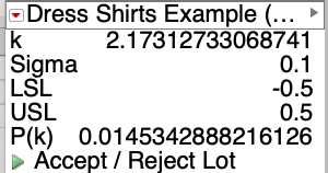
Just press the green Accept / Reject icon from the collections JMP data table to perform the necessary calculations and make a determination about the batch your sample came from.

One thing to remember about variables sampling plans is that only one measurement can be examined per sampling plan. So if you need to assess the length of sample handles on the coffee mugs, as well as, their performance ( how well they retain heat or keep your beverage cold ), two separate sampling plans are required. However, variables sampling plans require much smaller sample sizes than attributes plans.

RISKS WITH ACCEPTANCE SAMPLING

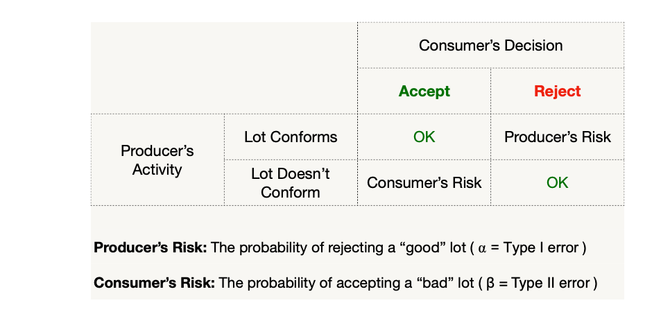
Because we are not sampling the entire lot, there are two types of risk that we must consider:

• The probability of rejecting a "good" lot or batch, also known as Producer’s Risk = α. 
• The probability of accepting a "bad" lot or batch, also known as Consumer’s Risk = β. 

Sampling plans Type 1 and Type 2 errors

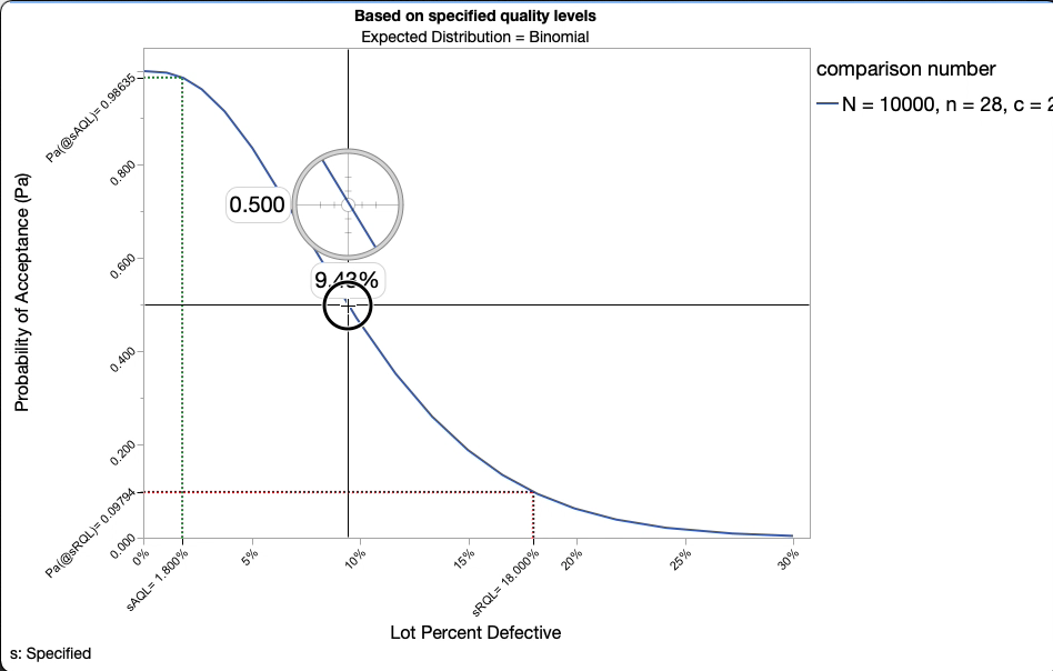
When you use JMP for acceptance sampling, the software produces many graphs.  One of the graphs produced are operating characteristic curves (OC curves) to quantify these risks. The OC curves illustrates the probability that a lot containing a certain fraction of defects or defective items will be accepted. The OC curves in the JMP sampling plan are shown based on both specified quality levels and specified probabilities of acceptance. 

Operating Characteristic (OC) Curves

In the graph on the left which is based on the specified quality levels and a sample size of 28 items, using the crosshairs tool we can visualize there's a 50% chance of accepting the batch when 9.43% of it is defective.

Crosshairs tool showing 50% probability of acceptance

Similarly, if the percent defective is 18% or (RQL), there's only a 9.79% chance of accepting the batch.

Over the next series of posts, I'll go through examples of acceptance sampling by attributes, zero acceptance sampling plans or Squeglia plans, variables sampling plans and double sampling attributes plans.   

JMP Acceptance Sampling Plan Add-In