What shape is a data table?

rcarver · Jun 26, 2018 09:59 AM

Reshaping data is one invaluable stage in the process of preparing a data table for further analysis and modeling. For most analyses, we organize data into a two-dimensional tabular format in which each row is an individual observation or case, and each column contains a measurement or attribute pertaining to that individual. There are times, though, when this is not the only option or even the preferred option.

Consider a simple pilot study for a controlled experiment. The experiment investigates the effect of a training activity intended to increase a subject’s score in performing a task. Suppose that the experiment is designed so that each subject in the study completes a pre- and post-test, and the scores are recorded. There are eight pilot subjects identified as individuals A through H, four of whom are randomly assigned to use the activity. The other four are the control group.

After data collection, we’ll have two scores for each person, and we’ll know which individuals were in each group. What are our choices for placing the data into a single matrix or data table?

Wide Versus Long Format

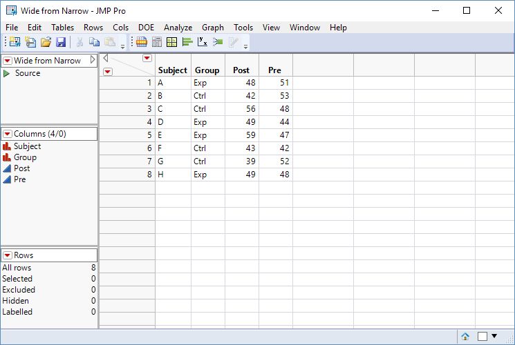
If we follow the convention of allocating one row per experimental subject, our data table might look like this:

Table 1: Wide Array of Artificial Experimental Data

Subject	Group	Pre	Post
A	Exp	51	48
B	Ctrl	53	42
C	Ctrl	48	56
D	Exp	44	49
E	Exp	47	59
F	Ctrl	42	43
G	Ctrl	52	39
H	Exp	48	49

This format is often referred to as “wide”: All of the attributes and measurements of a given individual are spread across several columns. In this example, we have a matrix of eight rows and four columns with minimal redundancy.

An alternative to the wide format is to rearrange the same data in a “narrow” or “tall” arrangement. This introduces some redundancy in the Subject, Group, and Test columns in exchange for treating the test (pre- or post-) as a categorical variable and treating all of the scores as a single numeric variable.

Table 2: Long Arrangement of the Same Data

Subject	Group	Test	Score
A	Exp	Pre	51
A	Exp	Post	48
B	Ctrl	Pre	53
B	Ctrl	Post	42
C	Ctrl	Pre	48
C	Ctrl	Post	56
D	Exp	Pre	44
D	Exp	Post	49
E	Exp	Pre	47
E	Exp	Post	59
F	Ctrl	Pre	42
F	Ctrl	Post	43
G	Ctrl	Pre	52
G	Ctrl	Post	39
H	Exp	Pre	48
H	Exp	Post	49

Ultimately, the decision about the preferred shape of a data table should be driven by the logic of your analytical goals. In designing an experiment or data collection from scratch, you should consider the analytical goals from the outset. Frequently, though, the layout of a data table was chosen at an earlier time by others, and the job of the analyst is to render the data into a format that suits the current purpose.

Reasons for Wide and Long Formats

Perhaps the most common reason for arranging data into a wide format is that we are working with longitudinal or repeated measures data. Some analysis platforms might require that each repeated measurement be treated as a variable. (See, for example, Grace-Martin 2015, or SAS Institute 2016a.) For some procedures, JMP can model repeated measures in either wide or long format, as discussed in SAS Institute 2016b. Because repeated measures of the same subject or observational unit are likely to be correlated with one another, they are better treated as multiple variables rather than a single variable.

When the analytical goal involves explicitly viewing time as a factor or predictor, as in time series modeling or visualization, then a long format might be more suitable. For example, a data table should be long to use the Time dimension on the JMP Bubble Plot platform.

The next two sections illustrate the JMP method for converting wide to narrow format and vice versa. The initial illustration uses this artificial data set only to present the method simply before moving on to more complex illustrations.

Stacking Wide Data

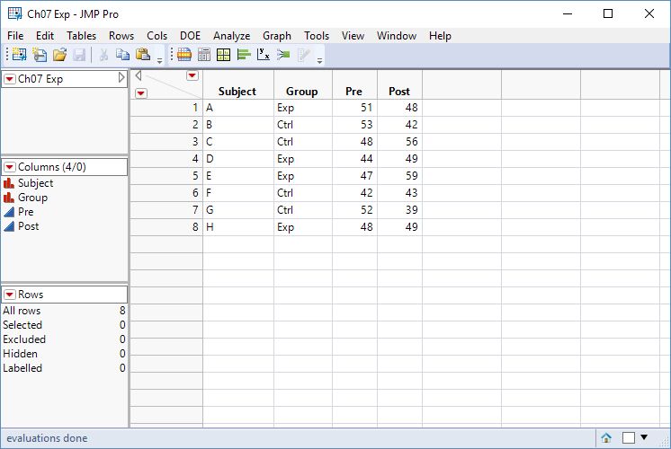
In this introductory example, the initial state of the data is wide with one row per subject and the two measurements occupying separate columns. In other words, the two measurements are being treated as two variables. Figure 1 shows the initial state of the data table. Because the design of this hypothetical study uses matched pairs, we might move directly to analysis with the data table.

For other analytical purposes, it could be helpful to reshape the table to the narrow format. We use the Stack command in the Tables menu.

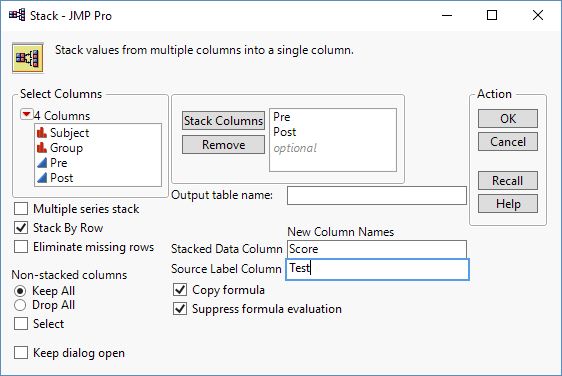
Figure 1: Example Data Table in Wide Format

Select Tables > Stack to open the dialog box shown in Figure 2.
The goal is to create a new column that represents the test administration as a categorical variable (pre- and post-) and stacks all of the scores into a single column. To do so, we select the two current columns (Pre and Post), and click Stack Columns.

By default, JMP will name the new quantitative column Data and the categorical identifier (that is, the original column names) as Label. It’s probably better to select more meaningful variable titles.

In the lower right of the dialog, specify a descriptive column title for the scores and for the experimental phase.
Complete the dialog as shown in Figure 2 and click OK.

Figure 2: The Stack Dialog

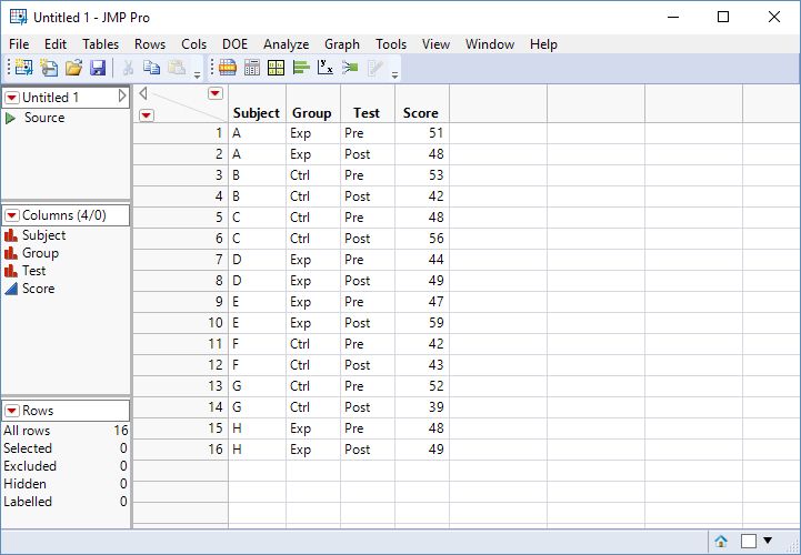
A new data table opens with the 16 measurements represented in narrow (long) format. Your data table should now look like Figure 3.

Figure 3: The Experimental Data in Narrow, or Stacked, Format

Unstacking Narrow Data

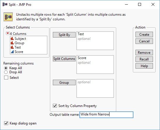
Suppose that the data were initially been recorded in the narrow format (similar to Table 2 and Figure 3), but we want to reorganize it in the wide format. To continue with the example and to reverse the process, we’ll use the Split platform in the Tables menu. The dialog appears in Figure 4. Here we need to specify the column that identifies the basis for unstacking (in this case, the Test column) as well as the column containing the data that will populate the multiple new columns.

By default, JMP will drop all columns except those chosen in the split specification. For this example, it will make sense to retain the information about the subject and the experimental group.

So click the button next to Keep All under Remaining columns as shown in Figure 4. The dialog also provides the option to rename the new wide table.
Complete the dialog as shown and click Create.

Figure 4: Split Table dialogThe results of this command appear in Figure 5. This nearly brings us full circle, with the one exception that JMP alphabetizes the order of the split columns. So, in contrast to Figure 1, the post-test data is now the third rather than the fourth column. You would need to note this in using the Matched Pairs platform for a pair-sample t-test or confidence interval. Since JMP 13, the Matched Pairs platform is among the Analyze > Special Modeling options. Veteran JMP users have previously found it in the Analyze menu.

Figure 5: The Experimental Data after Split to Wide Format

The content of this post is an excerpt of Chapter 7 of my book, Preparing Data for Analysis with JMP, where you will find more techniques for working with tables, and many more data cleaning tips.

References

Grace-Martin, K. (2015) “The Wide and Long Data Format for Repeated Measures Data”, available at http://www.theanalysisfactor.com/wide-and-long-data/.
SAS Institute Inc. (2016a) JMP 13 Fitting Linear Models. Cary, NC: SAS Institute Inc.
SAS Institute Inc. (2016b) “Sample 30584: Analyzing Repeated Measures in JMP Software” available at http://www.jmp.com/support/notes/30/584.html.