The stack mole

[#1]

Even though I’ve worked at JMP for more than 10 years, I’m still learning new things. Most recently, it was a new view of the Ishikawa diagram and the power of recursion. While both have been around for ages, it wasn’t until I had a specific challenge that I cared about them. This new motivation came when I was developing Geocoding 2020, an add-in that uses a REST API for communicating with a server. The data, coming from the server, was in form of a JSON array that could be quite large, depending on the data. One of the hidden gems in JMP (or more specifically, in JSL), is the command Parse JSON(), which translates a JSON array into a JSL list or associative array. It was a pretty good starting point, but still, if I wanted to grab specific parts of the data, I needed to know how to find and address them. Not an easy task if that array is made from several hundreds of items, deeply stacked in lists and arrays. So, I decided to write this helpful little program, stackmole.jsl, to give me an overview of the data structure. And, I wasn’t a respectable JMPer if I didn’t look for a graphical presentation.

Every server call could deliver data with a completely different depth, width and volume. The presence or absence of part of the data depends on the data itself. It’s impossible to know in advance what that data structure looks like. I needed a program that could decide for itself if it should go on looking for data, if it should look for the next list or array, or if it was at the end. Recursion was my answer to that problem. I know recursive definitions in mathematics, but how would that work in a data structure? Surprisingly well!

Data structures and recursion step by step

Recursion means that I apply the same rule or logic to the result that I produced the step before. The definition of a factorial of a whole number is the most widely known example. The factorial of a number is the product of that number with all the smaller numbers down to 1, which means the factorial of 3 is often written as 3! = 3 * 2 * 1 = 6. The Scripting Guide shows the statements for that routine:

myfactorial = Function( {a},
   If( a == 1,
       1,
       a * Recurse( a - 1 )
   )
);

Recurse can only be applied to a function; the command stands in the function itself and calls that function with the new argument. In the example of 3!, the function is called with 3 as the argument: myfactorial(3). Since 3 does not equal 1, the else clause of the IF statement is executed. This means multiplying 3 with the result of myfactorial (2). Again, that does not equal 1 and the else clause now multiplies 2 with the result of myfactorial(1). There is a result now; it is 1.

JMP remembers that the open task before was to multiply 2 with this result (2 * 1 = 1) and the task before that was to multiply 3 with the recursion result, which is 3 * 2 = 6. Since 3 was at the topmost level, the result is 6. The mechanism can be imagined as going down a stair. On every step, the open task is put down. The program goes down as many steps as necessary, until there is no more recursion. On its way back up the stairs, it collects all the tasks and ends up the starting floor with the result.

JSL knows some data collections, (e.g., variables that represent many values). The structures that can be analyzed by this program are lists and associative arrays. Lists are comma separated lists of elements such as:

list = {"a", "b", 1, 2}

Associative arrays are lists of key-value pairs.

assarr = ["a" => "This", "b" => "is", "c" => "a", "d" => "sentence"];

The first element of each pair is the key; the second is the value. Keys need to be unique and are internally sorted alphabetically.

Because of the different concepts, each structure needs different commands to change or read their content, they can be looked up in the Scripting Guide. What output would the stack mole produce from analyzing a simple list?

list = {"a1", "b1", "c1"};
stackmole (l);

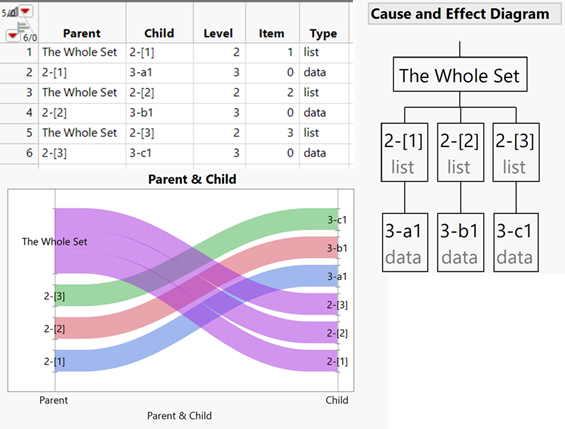
The data table is the list of items that the mole found when drilling down into the depth of the structure. The rows are to be interpreted from a child perspective. The whole set is a list, with the first child (on level 2) as the first item in that list. This child (row 2) is the data and its value is “a1”. Data is the endpoint of every journey, which means if there is no other item, the item is zero.

More informative is the Cause and Effect Diagram, which is the Ishikawa diagram in its hierarchical style. At the bottom, there are the data values above them their indices in square brackets. In this little example, the name of the whole set is “list”, so, if you want to get “b1”, it is list [2].

The parallel plot shows that the whole set splits up into three elements, and the next level elements no longer split up, since they contain the data. While it helps to understand small structures, at the end of this article, I’ll show a colorful parallel diagram that doesn’t help anything.

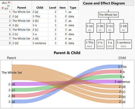
The results for an associative array differ slightly from the list report in that they contain the names of the keys:

sentencearray = ["a" => "This", "b" => "is", "c" => "a", "d" => "sentence"];
stackmole(sentencearray);

The type of the whole set is aa, which is short for associative array. The whole set is called “sentencearray”; if you want to access the word “sentence” in that array, do so with sentencearray [“d”].

This method is straightforward since it uses just one structure with a set of elements. But JMP allows to stack these structures in an arbitrary way and depth. So, you may have lists of associative arrays of associative arrays of lists, … In this example:

array = ["2list1" => {{"4list1_1", "4list1_2", "4list1_3"}, {"4list2_1", "4list2_2"} },
        "2list2" => {{"4list3_1", "4list3_2"}, "4element1" }  ];

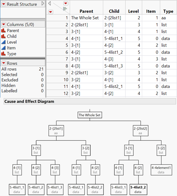
“array” is an associative array with two keys named “2list1” and “2list2”. The values of each key are lists, the first list again consisting of two lists, the second list consisting of a list and a data element. The numerals at the beginning of each term indicate the depth of the stack where those elements reside. In the analogy of the staircase, it is the number of steps that you need to go down to reach this element.

In this case, the stack mole delivers the following information:

The picture shows only part of the data table that now has 21 rows. The hierarchy diagram is complete. If you want to get to the data element 4list3_2 (in bold), the path is:

array["2list2"][1][2]

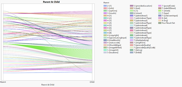
Below is an example of a parallel plot that doesn’t help at all, but still gives an interesting pattern:

The program has many comments that explain the single steps of the analysis and how the recursion is applied.