- JMP User Community
- :
- Blogs
- :
- JMPer Cable
- :
- Sometimes special data need special modeling tools. JMP® Pro Functional Data Exp...
- Subscribe to RSS Feed
- Mark as New
- Mark as Read
- Bookmark
- Subscribe
- Printer Friendly Page
- Report Inappropriate Content
Not all data contributing to a problem, or resulting from a process, are equal, such as functions, signals, spectra, or series defined over continuums like time, spatial location, and wavelengths. Sampling at points along the continuum (grabbing values from the curve) is possible, but not sufficient. These data require basis function expansion, a method for capturing non-linear relationships using a set of independent functions.
JMP Pro’s Functional Data Explorer (FDE) handles such situations. JMP Pro performs the magic under the covers, so users can deploy FDE interactively for exploratory data analysis, or for dimension-reduction to convert the functional data into a form that can be analyzed in another JMP platform.
JMP developers have designed all the model fits in the JMP Pro FDE platform to rely on basis function expansion, a method for capturing non-linear relationships using a set of independent functions. Want a quick overview? I created short videos about the models:
- A Deeper Dive into Basis Function Expansion Models for Functional Data Analysis
- A Deeper Dive into Wavelet Models for Functional Data Analysis.
Understanding how basis function expansion models are deployed in JMP Pro
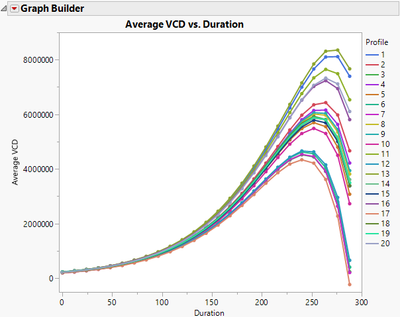
Functional data are collected over a continuum. The object of interest is an entire curve, not just one value from a curve. A sample of observations is a collection of multiple functions, as shown in Figure 1.
Figure 1. Multiple curves in a set of data.
Functional data analysis (FDA) extracts the essential shape information from the observations. Instead of summarizing interesting features of curves using variables that are probably highly correlated, FDA extracts independent variables containing the shape information. This information is contained in ordinary variables and can be used in other statistical analyses.
The models used to extract the shape information are linear combinations of basis functions. That is, the model is the sum of coefficients times basis functions, as shown in Figure 2.
Figure 2. Basis function expansion modeling.
JMP Pro offers different types of basis function expansion models: B-splines, P-splines, Fourier basis functions, and wavelets. Each uses different basis functions. For example, basic splines, or B-splines, use basis functions that are piecewise polynomial functions. A model selection criterion is used to choose the degree of the polynomial. Penalized splines, or P-splines, also use piecewise polynomial functions for the basis functions, but their pieces are put together differently than the B-splines. Fourier basis functions are pairs of sine and cosine functions with different periods. Wavelet models use complex functions that can model all types of data, including those with sharp peaks, like in spectroscopy data.
The platform provides graphs to help interpret the fitted models, starting with the shape functions, as shown in Figure 3.
Figure 3. Shape functions.
These shape functions can be used to understand the curve-to-curve variation in the data around the mean. They indicate the shape features of the data curves. The basis function model can be rewritten as a linear combination of shape functions. The coefficients of the shape functions are the functional principal component scores. These functional principal components are new, scalar variables that contain the shape information in the data. They are uncorrelated with each other and can be used as responses or factors in other statistical analyses.
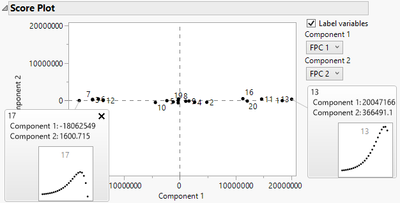
Plotting the functional principal components can help with model interpretation. With JMP’s hover graphlets, it’s easy to see the differences in the data curves across the values of the functional principal components, as shown in Figure 4.
Figure 4. Score plots comparing functional principal component values for two curves.
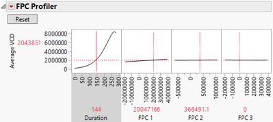
The Functional Principal Components (FPC) Profiler helps interpret how changing the coefficients of the shape functions changes the predicted shape of the curve, as shown in Figure 5.
Figure 5. FPC Profiler for interactively approximating the curve using FPC coefficients.
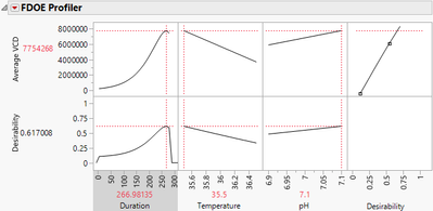
A linear combination of the shape functions can be used to approximate each function. The coefficients of the shape functions in the linear combination are the functional principal components. Saving the functional principal components gives new scalar variables than can then be analyzed using any ordinary statistical analysis, including as responses in a designed experiment, as predictors in a statistical model, control charts, gauge studies, cluster analysis, among many other techniques, as shown in Figure 6.
Figure 6. Optimization in the FDOE Profiler using a functional DOE model for the curve response.
Understanding wavelet basis function models
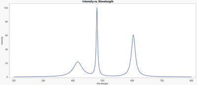
Wavelet basis function models work very well to model data of any shape, and are especially good at fitting data with with sharp peaks, such as curves found in spectral analysis, as shown in Figure 7. Their main weakness is that they need at least 10 observations per function, so are not suitable for modeling short functions.
Figure 7. Simulated spectral data.
Wavelets are functions which oscillate above and below the X axis, so they integrate to zero. They decay quickly on the edges, as shown in Figure 8.
Figure 8. Example wavelet function.
JMP Pro offers a selection of models from five families: Daubechies, Haar, Coiflet, biortogonal, and symlet. The family is defined by the mother wavelet.
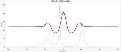
The model consists of the sum of two linear combinations. The first is a linear combination of scaling functions and contains no shape information. The second is a linear combination of coefficients times basis functions. The first part of this linear combination is a coefficient times the wavelet stretched to the domain of the function, as shown in Figure 9.
Figure 9. Wavelet applied to the whole domain.
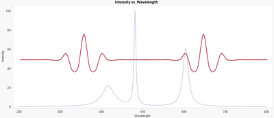
The second part cuts the domain in half and has two coefficients times the wavelet stretched to the first half and the second half of the domain, as shown in Figure 10.
Figure 10. Wavelet applied to both halves of the domain.
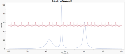
Next, the domain is cut into fourths, then eighths, and so on, as shown in Figure 11.
Figure 11. Wavelet applied to 25 segments of the domain.
The coefficients of the wavelets at different resolutions from cutting the domain into 2j segments will be large when the frequency of the wavelet matches the frequency of the data and small when the frequencies don’t match. Also, because the wavelets decay on the edges, they are localized to their domain, and thus can model sharp peaks very well. Recall that Fourier basis functions are sine and cosine pairs whose peaks are not localized. They vary over the entire domain of the function, so they are not able to model sharp peaks very well.
The approximation at step j + 1 is :
The values of phi are the scaling functions and the values of psi are the wavelet functions. The size of the function needs to be a power of 2 to fit the wavelet model. JMP Pro expands the domain as needed. Also, the data need to be on a regular grid. JMP handles this as well, automatically performing a Cleanup > Reduce > Grid. At each stage, JMP performs Lasso shrinkage of the wavelet coefficients, so small, meaningless coefficients can be replaced by zero.
You must be a registered user to add a comment. If you've already registered, sign in. Otherwise, register and sign in.
- © 2024 JMP Statistical Discovery LLC. All Rights Reserved.
- Terms of Use
- Privacy Statement
- About JMP
- JMP Software
- JMP User Community
- Contact

