JMPer Cable
A technical blog for JMP users of all levels, full of how-to's, tips and tricks, and detailed information on JMP features- JMP User Community
- :
- Blogs
- :
- JMPer Cable
- :
- Replicating Pandas GroupBy behavior in JMP
- Subscribe to RSS Feed
- Mark as New
- Mark as Read
- Bookmark
- Subscribe
- Printer Friendly Page
- Report Inappropriate Content
The Engineering Mailbag
Episode 4: Pythons and Pandas, Oh My!
Every now and again we systems engineers run into interesting questions that would fall somewhat outside the typical range of JMP usage. These applications are generally clever, and often bring home how using data isn’t limited to solving business or technical problems. Other times, the questions are just unexpected, challenging problems. These “curve balls” (as I like to call them) come in many different forms: coding problems, interesting analyses, ways of visualizing data… you get the idea.
I haven’t written from the mailbag in a while, but this particular question really seemed to be something that needed to be addressed. The tool I used to answer the question really isn’t discussed as much as I think it should be. So, this is an opportunity for me to help out a colleague from New York and show everyone something interesting that you might not be aware that JMP can do.
The Question
Mike[JMP],
Often, I need to do groupbys where I need to grab say the max value everything grouped by some label where the Python Pandas equivalent would be something like:
df.groupby(['Something', 'Something Else']).max()
Another might be something like pandas.nlargest with a groupby, where I would want say the top 5 things out of a groupby.
And after a couple minutes of fiddling with a column formula I give up and export the data to reimport it into JMP later. Tabulate sort of does this, but not always in the way I want. So a "How to JMP like Pandas" document would be super helpful for me, and might be helpful for JMP with how widespread Pandas has become…
Thanks,
Nick
My Response
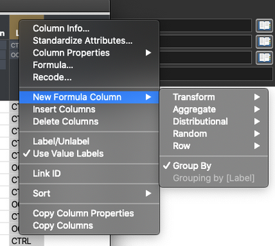
Hi, Nick!There is a trick that you can use to get more flexibility out of formulas that mimics a lot of what [Pandas] can do. It involves telling JMP what columns you want to group by. You do this by right clicking on the column name and selecting New Formula Column > Group By.
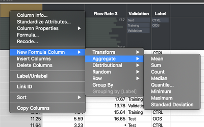
After doing that, any formula columns you create by right clicking on the column name and using New Formula Column> … will be grouped by the grouping columns you set.
After that, it’s just a matter of filtering or subsetting using data filters or local data filters. Let me know if that helps!
Best,
M
Pandas: Cute Mustelid or Data Analysis Tool
All right, for the uninitiated, Pandas is not a cuddly, chromatically challenged mustelid. Pandas (usually abbreviated as “pd” in python scripts) is a “…Python programming language for data manipulation and analysis. In particular, it offers data structures and operations for manipulating numerical tables and time series [source]." It basically fills the role that the data organization and manipulation parts of JMP (data tables, Row and Column menus, etc.) do in the Python programming environment. So, it’s pretty important to Python data analytics workflows. Now, if you are looking to run Python from within JMP, this ain’t the blog article for you. Go have a look at this white paper. If you are looking to break yourself free from doing data transformation in a command line, read on.
DataFrames and Data Tables
Still here? Awesome. Okay, the rest of this article is going to go through some of the common bits of Pandas and their analog in JMP. It’s not a comprehensive list by any means; it’s intended to point your nose in the right direction when thinking about the two environments.
The first bit I want to cover is the “DataFrame.” In Pandas, this is where everything is stored. Like data tables in JMP, it is essentially a collection of data columns with a name (column name), etc. You act on columns and rows (transform things, summarize, etc.) but you’re always acting on either the DataFrame as a whole or some part of it.
In JMP, the primary data container is the data table. You can act on columns and rows in the same ways you would in a Pandas DataFrame. In both, you are able to deal with missing values in the data table. In JMP, they are designated as either a cell with a “.” in it (for numerical data) or a blank cell (for character data). You can transform data, summarize it, etc. (more on those bits later). In both cases, the more you tell the software about the data the less leg work you have to do, which brings me to my next point.
Column Properties and dtypes
In the matter of column properties and data types (dtypes in Pandas), JMP wins hands down. Pandas inherits most of its data type understanding from another Python package called NumPy, which is cool. NumPy is pretty sturdy code, but it’s really limited in this regard. It handles about eight types of data (see the table below[source]) with somewhat limited support for different formatting (it gets pretty confused by currencies without help, for instance).
|
Kind of Data |
Data Type |
Scalar |
Array |
String Aliases |
Documentation |
|
tz-aware datetime |
'datetime64[ns, <tz>]' |
||||
|
Categorical |
(none) |
'category' |
|||
|
period (time spans) |
'period[<freq>]', 'Period[<freq>]' |
||||
|
sparse |
(none) |
'Sparse', 'Sparse[int]', 'Sparse[float]' |
|||
|
intervals |
'interval', 'Interval', 'Interval[<numpy_dtype>]', 'Interval[datetime64[ns, <tz>]]', 'Interval[timedelta64[<freq>]]' |
||||
|
nullable integer |
Int64Dtype, … |
(none) |
'Int8', 'Int16', 'Int32', 'Int64', 'UInt8', 'UInt16', 'UInt32', 'UInt64' |
|
Strings |
'string' |
||||
|
Boolean (with NA) |
'boolean' |
The column properties in JMP comprise about 43 pages of the Using JMP book. They are significantly more extensive and are good at recognizing data types as they are imported. Of particular interest to a new JMP user is the fact that column properties extend well beyond the data types that Pandas uses. It can handle a host of metadata that trigger actions across the software. Now, to be fair, you can attach attributes to a Pandas DataFrame, but since the DataFrame is just a container, you have to either code in the support for the attributes or hope someone put in the support in the package you are using. All that is already done for you in JMP.
Tabulate, Column Formulas and GroupBys
The truth is that the previous two items don’t really matter that much in the context of the question I was trying to answer. For our purposes, the data table/ DataFrame is just a box to put stuff in. The column properties/types can help with analytical considerations, but, again, that’s not important for the question we’re working with here. The bit of Pandas that we are interested in is called GroupBy. And it’s for slicing and dicing data in preparation for doing other analyses. A quick example using the JMP Big Class data table and getting the average height and weight of boys and girls by age might look like this:
# Import Pandas
import pandas as pd

# Bring in the data
data = pd.read_csv("/Users/mike.anderson@jmp.com/Desktop/Big Class.csv")

# Put the data into a DataFrame
df = pd.DataFrame(data)

# Run the group by, get the means, and show the results
summ_df= df.groupby(['sex','age']).mean()
print(summ_df)
With the output looking something like this:
          height   weight
sex age
F  12  58.600000 100.200000
  13  59.000000  95.333333
  14  62.600000  96.600000
  15  63.000000 102.000000
  16  62.500000 113.500000
  17  62.000000 116.000000
M  12  57.333333  97.000000
  13  61.250000  94.250000
  14  65.285714 103.857143
  15  65.200000 110.800000
  16  68.000000 128.000000
  17  69.000000 153.000000
Normally, JMP users would look to Summary or Tabulate as their primary tools for these data transformation operations. They might even use the Formula Editor to create a column. But, there is a secret weapon in the data table (and in the platform column list) that you can use to do just about everything you’d want to do in Pandas and more. That secret is the ability to right click on a column name and select New Formula Column. This works anywhere that there is a column list! From there you have many different options for doing various transforms, such as combining columns, doing cumulative sums in rows, etc. That, in and of itself, while handy, is not particularly magical. The place where things get really interesting is when you turn on the “Group By” flag for a column in JMP. This will automatically make any formula columns you create aware of the levels in a grouping variable. Just think about that for a second -- you can create a formula column anywhere in the software that can be stratified based on a grouping column.
Let’s look at an example of what this means from another question I received recently:
An Example: TWO QUESTIONS FOR THE PRICE OF ONE!!
About the same time the initial question came through, I got a question from another customer about how to do a numerical integral (area under a curve or AUC) for a large collection of samples. Moreover, they were willing to provide me with a sample data set they had published previously for a journal article in Environmental and Molecular Mutagenesis.
It turns out that what they wanted to do was easily accomplished using Group By Flags and Function Columns. Here’s the procedure (you can follow along using the data from the JMP Public site:(
First, let’s graph the data. The details of the study aren’t important for this discussion, though it is interesting reading. The short version is that it’s a large collection of chemicals with different concentrations (Conc. (uM)) and a series of genetic responses. For our exercise, they’re interested in calculating the AUC for each of the genetic responses. Here’s a look in Graph Builder with a column switcher:
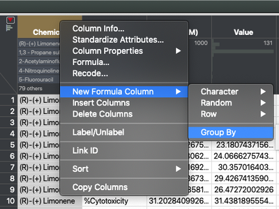
The first step in the process of calculating the AUC is setting up the grouping. We’re going to right click on the Chemical column, select “New Formula Column,” and then “Group By.” We’re going to do this again for the Biomarker column. Note that order can matter here. We’re grouping first by Chemical and then Biomarker within Chemical. After that, it’s just a matter of using the “New Formula Column” in the data table to build up the calculation.
Going forward, I broke each step out into individual columns for the sake of clarity. And, if you’re really interested, I’m using the Trapezoidal Rule Riemann Sum for the math here.
Ok, back to the calculation. The first thing we need is the distance between each point in the x-axis (the point-wise change in x). We’re going to select the Conc (um) column, right click on the title and select New Formula Column>Row>Difference. Now open the formula in the new column that JMP created. It should show something like this:
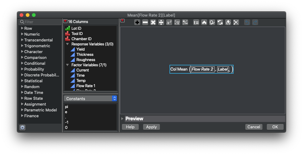
Note that JMP is handling calculating between rows and has adjusted the formula to reset when it detects a new Chemical or a new Biomarker type.
Next we need the average value of Value between each data point and the previous one. Right click on the column header and select New Formula Column>Row>Lag. Open the formula and modify it a little so that it’s calculating the difference between rows and not just giving the value of the previous row. That’s shown in this screenshot:
Those two columns (I renamed them dx and dy in the data table) need to be multiplied together to get the area of a segment. Select the two columns, and right click on the column name of one of them. Select New Formula Column>Combine>Product. The new column gives us the approximate area under the portion of the curve between each data point and the next one. I renamed that column iAUC(for instantaneous AUC) in the data table.
The last step is to sum up the values for each section. This is done by right clicking on the iAUC column and selecting New Formula Column>Row>Cumulative Sum. Because we selected the Group By columns at the beginning of the exercise, the tally is reset for each sample in the data set.
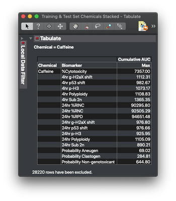
From here we could use Tabulate or Summary to create a table with the max values for each sample (the approximate total area under the curve). Here’s an example for a common chemical:
Final Thoughts
And, that’s it. You can easily replicate behaviors in Pandas using structures that exist in JMP. Just remember to use the Group By variable and you’re off. No mustelids, chromatically challenged or otherwise, required.
Editor's note: Have you read the other installments in our Engineering Mailbag series? See how Mike helps a user who was using JMP to decide whether to sign up for a snow removal service and develop unique visualizations for STEAM education programs.
- © 2026 JMP Statistical Discovery LLC. All Rights Reserved.
- Terms of Use
- Privacy Statement
- Contact Us




You must be a registered user to add a comment. If you've already registered, sign in. Otherwise, register and sign in.