- New to JMP? Let the Data Analysis Director guide you through selecting an analysis task, an analysis goal, and a data type. Available now in the JMP Marketplace!
- See how to install JMP Marketplace extensions to customize and enhance JMP.
JMPer Cable
A technical blog for JMP users of all levels, full of how-to's, tips and tricks, and detailed information on JMP features- JMP User Community
- :
- Blogs
- :
- JMPer Cable
- :
- Optimizing film topology using target functions in functional data analysis
- Subscribe to RSS Feed
- Mark as New
- Mark as Read
- Bookmark
- Subscribe
- Printer Friendly Page
- Report Inappropriate Content
Earlier in this blog series, I mentioned that functional data analysis (FDA) could be used with experimental design. It’s an interesting idea to consider. What if you wanted to optimize the shape of a curve? Or, understand how to control the periodicity of a response? That’s what I want to discuss in this last entry in this series. To do it, we’re going to use “The Way Back Machine” and go back to 2010 to that year's JMP ENBIS Challenge.
The 2010 ENBIS Challenge What's Golden Curve optimization or analysis?
Let me take you back to 2010. Ian Cox (@ian_jmp Worldwide Technical Director) submitted a simulator for an LPCVD (Low-Pressure Chemical Vapor Deposition) process to the European Network for Business and Industrial Statistics (ENBIS) annual conference for their ENBIS Challenge. The challenge was to find a process recipe that would maximize the simulated profit and reduce defectively on the simulated parts. If you want to play with the simulator, it’s still up.
Part of the challenge was that you had to consider the cost of development in the profitability calculations and only had a certain amount of total material to play withal (for production and development). I stumbled into the simulator a couple of years after the fact while I was looking for an example I could use for some training purposes. It turns out Ian did his homework when developing the simulator, and it does a nice job of replicating the output of the LPCVD process with realistic defect rates, etc. It’s still an informative tool for demonstrating why DOE is the only way to do process development. We’re going to use it here, although maybe somewhat outside its original scope.
Golden Curves Ahead
One of the main benefits of FDA is that it makes it possible to use curves (not individual data points) as factors in a model. One could also argue that we would want to look at how process factors (time, temperature, etc.) affect an observed curve. FDA can do that, too. The next logical step in that line of thinking is: I know the curve I’m after (either through first principles or process constraints). I want to optimize my process conditions to fit the curve I’ve provided as closely as possible. This idea is an extension of what we would do in JMP with the Profiler and the Maximize Desirability routine. In the world of FDA, that is called a “Golden Curve” optimization. This Golden Curve Analysis is what we are going to focus on today.
The Process
First off, I’m not going to give a long-winded treatise of LPCVD. It’s not that important to this discussion. But, just so you’re not flying blind, here’s the elevator speech version. The process is used to put films and coatings on stuff. The films can be functional (corrosion protection) or decorative (like finishes on higher-end bathroom fixtures). In LPCVD, you put a substrate into a chamber (this could be a silicon wafer, a drill bit, or the faucet in your kitchen). The chamber is then evacuated (the low-pressure part) and heated up to some temperature. Then reactive gasses are introduced into the chamber at a controlled rate. The gasses react and attach themselves to the surfaces of the parts. Some times radio frequencies are used to break chemical bonds in the gases to make the process more efficient.
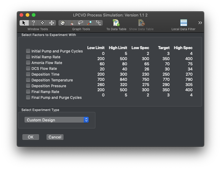
In the DOE simulator, we have control over a number of the process parameters and gas flow rates. The simulator gives data measured from 49 sites across the substrate arranged as a center point and three concentric rings of measurements. This measurement pattern is relatively standard in the industry. It’s not my favorite by a long shot, but it shows up a lot.
The Problem
There are a couple of problems we have to deal with in the LPCVD simulator. First is the issue of getting the target thickness and film parameters correct. If you didn't care about the profile of the film, this could be done using a standard DOE and focusing on some summary statistic like the average or median film thickness. The second issue is that, because of the geometry of the chamber and the way the gases flow, the film is not uniform. It usually has a toroidal feature in the middle of the substrate. This second problem is why we need to use FDA to deal with the analysis.
The Analysis
Let me skip ahead to the bit where I'm analyzing the DOE results. Doing a graphical analysis of the DOE wafers, we can see that the non-uniformity of the wafer has radial symmetry. We can use this to our advantage and convert the (x,y) coordinates provided by the simulation to calculate the radius for each point using the Pythagorean Theorem. This transform reduces the dimensionality of the data set and makes FDA more straightforward.
Before I do the FDA in the Functional Data Explorer platform in JMP Pro, I need to add a set of data to the DOE analysis results. This data set will be the target curve. It contains the target parameters for a large number of radii between the measured data points. I'm providing a large number of data points to force the optimization algorithm to look for a solution that matches the target curve (in this case, a uniform value across the substrate) closely.
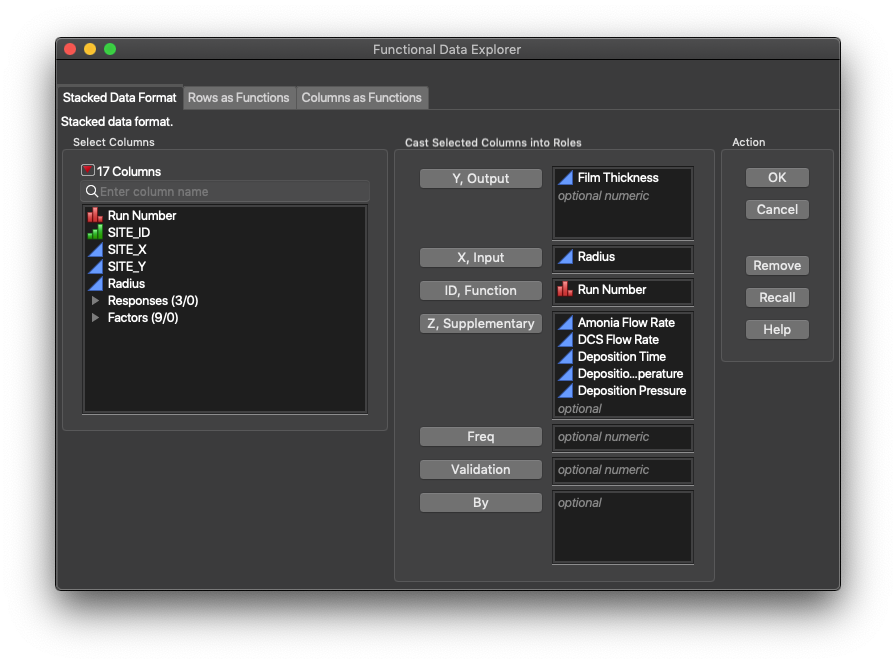
Now, I can do FDA. The setup in JMP Pro is below. I’m focusing on just the thickness in this example. Note that I’m using radius as my “X, Input” value. Recall in an earlier post in this series that the definition of time is somewhat fluid in FDA, so this is OK. Note that my DOE parameters are supplementary variables. Once I’ve hit OK in the launch dialog, I need to do one thing differently than I usually would with FDE. I need to click on the “Load” button in the Target Function part of the FDE interface. Doing this will bring up a dialog that lists the function IDs. I select the one associated with the target function (added when I created it) and click “OK.”
Now, with the preliminaries over, we can create the functional form of the experimental data and pass it to a modeling platform. There’s a good tutorial on how do the mechanics of creating the functional form here. JMP Pro 15 handles all the mechanics of passing the functional forms and the supplementary variables to the Fit Model Platform behind the scenes. So, you only need to select Functional DOE analysis from under the red triangle menu for the model. This will give you access to the Generalized Regression personality in Fit Model and pull up the Profiler automatically from within FDE. (Note that all the reports and data are available here on JMP Public.)
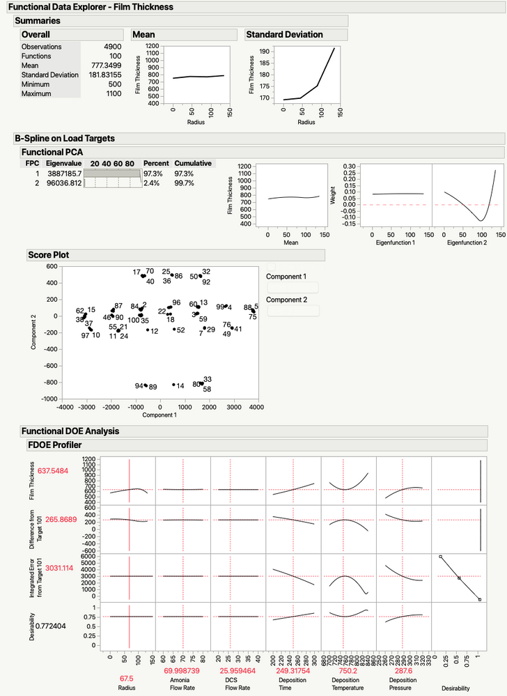
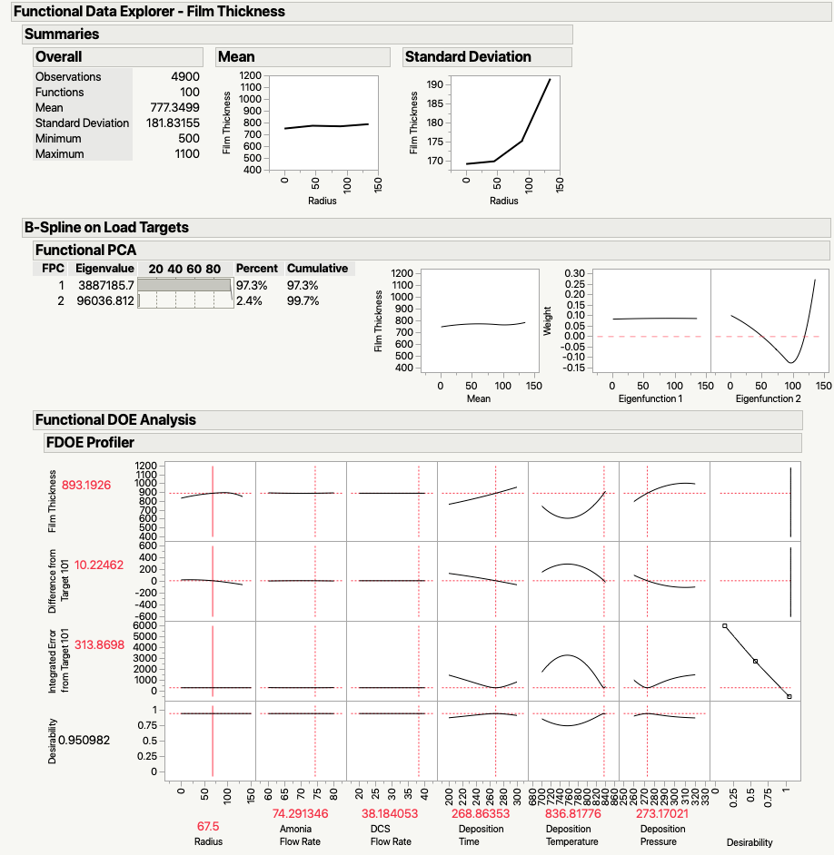
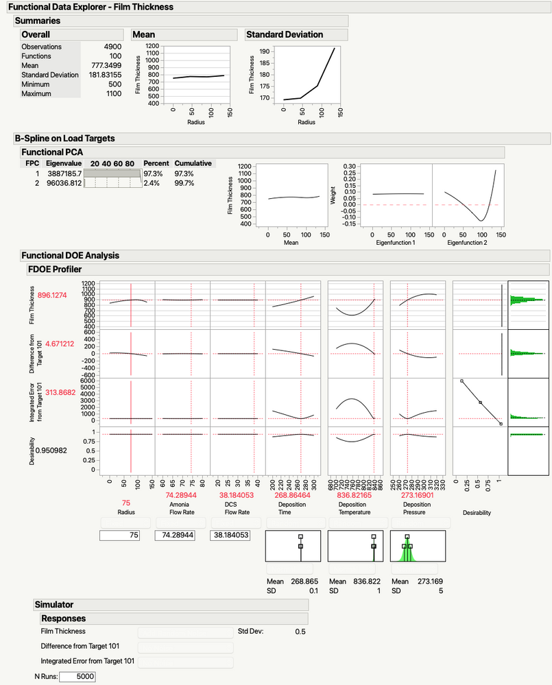
When you’ve provided a target function, the Profiler has two additional rows of graphs. These show the difference between the function produced by the current settings and the target function and the integrated error between the target function and the current function. When you select Maximize Desirability from the Profiler red triangle menu, JMP attempts to minimize the integrated difference between the target and the displayed function. In our case, JMP searches for the setting that produces the flattest thickness curve in the process. From there, you’d need to read off the values in the Profiler and do a couple of verification runs to check the results. (Always verify your DOE predictions, people!!).
Let's Practice What We Preach
So, looking at the FDOE Profiler, we can see that the parameters that really drive this process are Deposition Time, Deposition Temperature, and Deposition Pressure. We are going to presume that we need to run the process at 300℃, deposit for 824 seconds at 261 mTorr. However, there is a great adage involving assuming and what it turns oneself into ... so we're going to do some validation runs with those settings.
Before I do the runs though, I'm going to do a little simulation using the Profiler's simulation capabilities to understand the probable range of the data. I'm going to do that to act as a stand-in for a calculated confidence interval. It's not perfect, but it will at least give me an idea of what the output data should look like for this situation if my model is correct. Here's the FDOE output with the simulator turned on and some best guess values for the process parameters.
And, here are the results of the validation runs with some historical data from the ENBIS challenge for comparison. Note that this control chart is looking at the average film thickness over the entire wafer. If you look at the Profiler above, you can see that the edge and outer region of the wafer have lower film thickness. They also have the majority of the data points in the wafer (look at the sampling plan at the top of the article). This will combine to skew the wafer mean values downward (one of the major reasons I'm not a fan of this sampling plan). But, that little quirk aside, the wafers are now all within spec and the variation lot to lot has also dropped.
Conclusion
Golden Curve Analysis is probably my favorite application of FDA. Trying to optimize a process with a known spatial correlation while ignoring the effects of that correlation has always bugged me. However, it’s quite a challenge to do the analysis other ways -- particularly within the framework of a DOE.
- © 2026 JMP Statistical Discovery LLC. All Rights Reserved.
- Terms of Use
- Privacy Statement
- Contact Us

You must be a registered user to add a comment. If you've already registered, sign in. Otherwise, register and sign in.