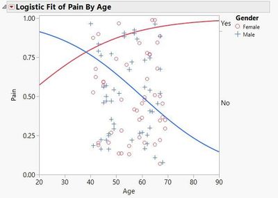
 Odds ratios in a logistic regression model are used to interpret the effect of the factors included in the model.
Logistic regression models are widely used throughout industry and academia. They are appropriate when one is attempting to model a binary response (Yes/No, Live/Die, Good/Bad…) or an ordinal response where ordering of the levels is important (Good/Better/Best, Mild/Moderate/Severe, etc.) Odds ratios in these models are used to interpret the effect of the factors included in the model.
Odds ratios for interaction terms are more difficult to compute and to interpret because of the properties of the odds ratio. With an interaction term, there is no single odds ratio. To get an odds ratio for one of the main effects involved in the interaction, you must define a fixed level of the other effect. That is, if you want an odds ratio for an effect A, when the interaction term A*B is included in the model, you must fix the level of B to compute the desired odds ratio.
Analyses in JMP are no different. To demonstrate, let’s look at an example. The (simulated) data shown below was collected from 100 individuals, measuring their Gender, Age, and if they have experienced low back pain in the prior six months.
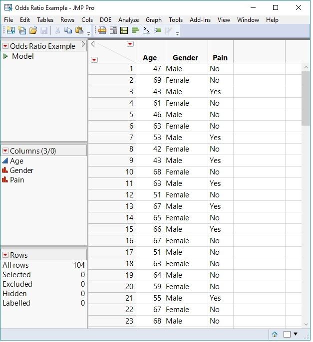 Partial display of the data collected.
Fitting the Model
In this simple example, a logistic regression model can be fit with “Pain” being the response variable, and the effects included in the model are “Age,” “Gender,” and the “Age” by “Gender” interaction term. The interaction term is included because the belief exists that as age increases, males and females do not respond the same. The response level Pain=”Yes” will be modeled as the event of interest. This model can be set up in JMP by selecting Analyze—>Fit Model and defining the terms as shown in the launch dialog below. Note that the response column “Pain” has a Nominal Modeling Type. This designation is necessary for the analysis.
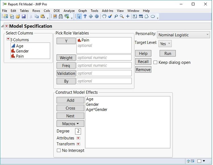 Defining the Logistic Regression model.
From the results shown, select “Save Probability Formula” from the Nominal Logistic Fit pop up menu. This selection will generate new columns in the original data table:
Lin[Yes] – The linear predictor, or the predicted logit function
Prob[Yes] – The predicted probability of the response being “Yes”
Prob[No] – The predicted probability of the response being “No”
Most Likely Pain – The predicted level of the response
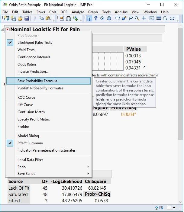 Saving the Probability Formula.
Obtaining the Odds Ratios
Formulas will be associated with each of these columns. In order to obtain customized odds ratios, create new rows in the data table defining the comparison settings. Here, there is interest in determining the odds ratio of 55-year-old males versus 65-year-old males, and 60-year-old males versus 60-year-old females. See the data table below to see the additional rows with the formulas described above evaluated.
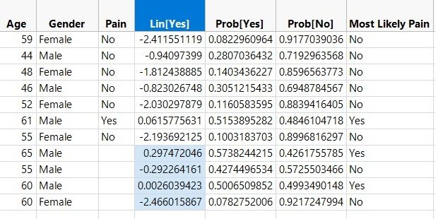 Added rows to compute customized odds ratios.
Now, the first odds ratio is computed as:
OR = Exp(0.297472046-(-0.292264161)) = 1.8035
This odds ratio of 1.8035 indicates that the odds of pain increase by a factor of 1.8035 for males as age increases from 55 to 65.
The second odds ratio of interest is computed as:
OR = Exp(0.0026039423-(-2.466015867)) = Exp(2.46861981) = 11.8061
This odds ratio of 11.8061 indicates that the odds of pain for 60-year-old males is 11.8061 times higher than for 60-year-old females. For a more detailed description of odds ratios, please review the JMP 14 online documentation on this topic.
These computations demonstrate a method of obtaining customized odds ratios for logistic regression models using JMP software. This method is not limited to interaction terms only; it can be used with main effects. So, the default odds ratios given in JMP may be just fine in some situations. In many cases, the tests of interest must be defined by hand, and the method described here will always get these tests of interest.