There are quite a few great new capabilities in JMP Pro 18: updates to GLMM; more genomics capabilities; mixed models and response screening for big data; and updates to SEM, to name a few. But if I had to pick just one new feature that I’m especially excited about, it would be the Peak Finding capability in the Functional Data Explorer (FDE).
Why is Peak Finding important?
Many companies have chromatographic and/or spectral data. Being able to analyze these data easily and natively in JMP Pro has been a common request for quite some time.
When you show FDE to R&D and manufacturing users in the biotech and pharmaceutical industries, they immediately see chromatographic applications. There are specific quantities users need to extract from the data – such areas under the curve (AUCs) and resolution metrics – that require a way to identify and label the peaks within a set of chromatograms. These quantities, which are used as part of process development, are critical for manufacturing and meeting regulatory requirements. There is, of course, specialized equipment and software for analyzing peak data and reporting these quantities, but time and time again, JMP customers have told us they wanted more of this natively within JMP, as this is where the data ends up being analyzed anyway.
How do I use Peak Finding in JMP Pro?
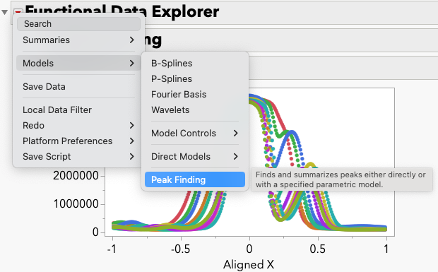
Peak Finding option in the FDE Models menu
I’ll go through a simple example using a chromatographic data set from our colleague Ben Barroso-Ingham’s doctoral research. A screenshot of the chromatographic data in FDE is below.
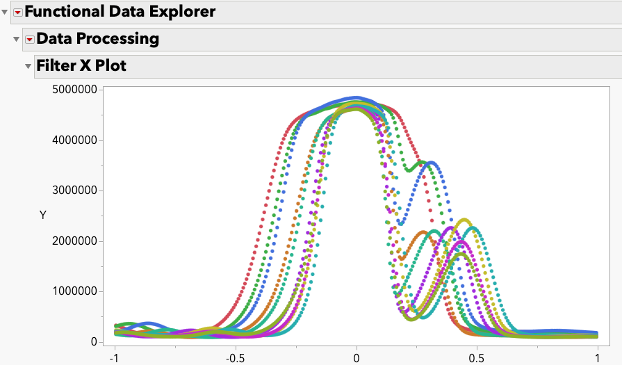
I already used some of the preprocessing tools in FDE so that we can focus on the most important part of the chromatograms. Ben ran a designed experiment on the settings of the chromatographic equipment that sought to separate the product compound, which corresponds to the larger peaks on the left, from an impurity that corresponds to the peaks on the right.
Ben varied two factors in his DOE: the temperature of the material in the chromatographic column and the flow rate setting of the column. The factor settings are seen in the screenshot below.

We can use the Peak Finding tool in JMP Pro 18 to identify and label the peaks, and then extract the resolutions of the peaks, which measures how well the peaks are separated from one another. Then, we can analyze those resolutions as responses with DOE statistical modeling tools like Generalized Regression.
To do this, we use the Peak Finding option in the Models menu in FDE.
We can now use the new Peak Editor. It has two tabs for viewing the data: a Single tab that lets you see the peaks for a single
chromatogram, and a Multi tab that lets you see them all together. What you see below is the Multi view for all 10 chromatograms.
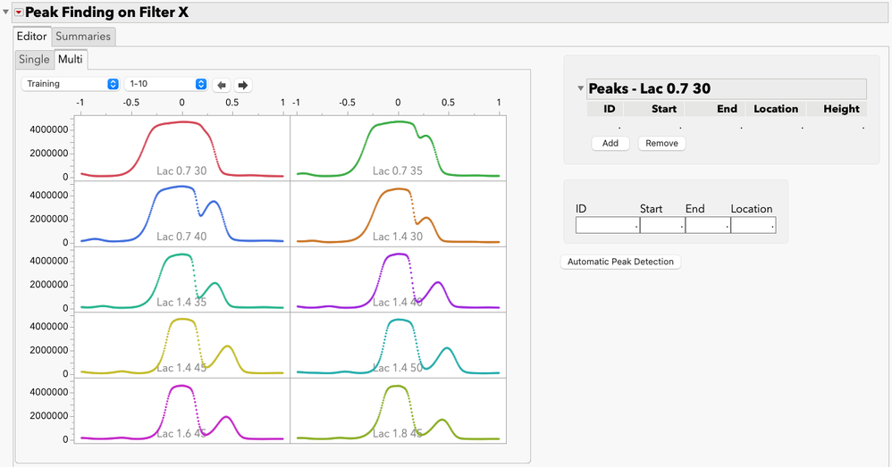
The goal here is to identify the peaks and label them so that we know which peak is which in each of the individual chromatograms. Once this has been done correctly, you can pull out the relevant features, such as the AUCs and resolutions from the Summaries Tab. This is not unlike the results of a Functional Principal Components analysis in previous versions of JMP Pro, but the summaries here are specific to peak-type data.
Finding the peaks
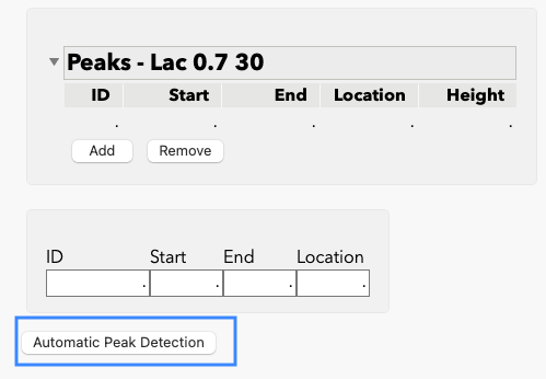
We use the Automatic Peak Detection option to do as much of the work as possible in terms of finding the peaks in the data and labeling them. While our goal is to make this peak-finding process as automatic as possible, we also know that no fully automatic solution will ever get the right answer 100% of the time. So, we hope that the Automatic Peak Detection will get you 90% of the way there, and then you can tweak the results as needed.
Here, I’ve clicked on Automatic Peak Detection, and you can see that it has found one to three peaks per chromatogram.
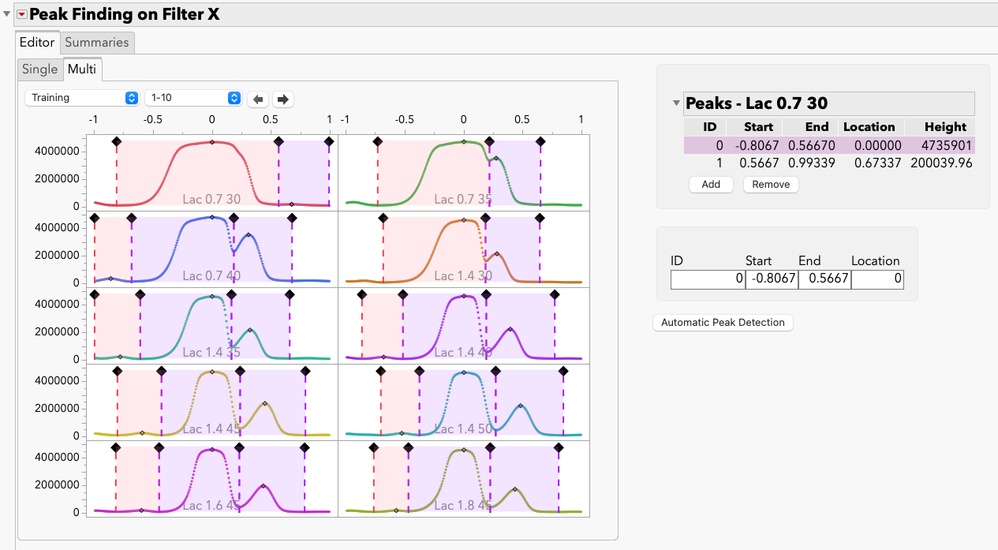
In some of the chromatograms, the Peak Detection has found small peaks we are not currently interested in. We can remove those peaks by going to the Single view, selecting the peak, and clicking Remove.
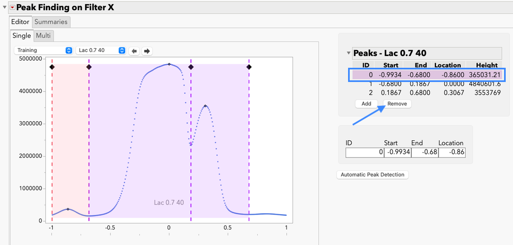
This is the result of removing peak “0” from the third chromatogram.
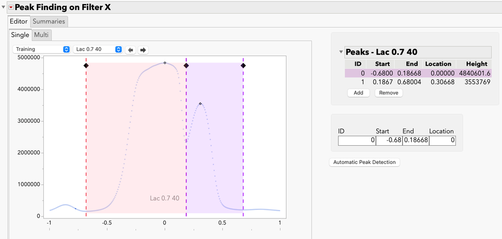
You can also add peaks and adjust their ranges by moving the dashed red lines. Alternatively, you can manually enter the ranges in the numeric entry box on the right.
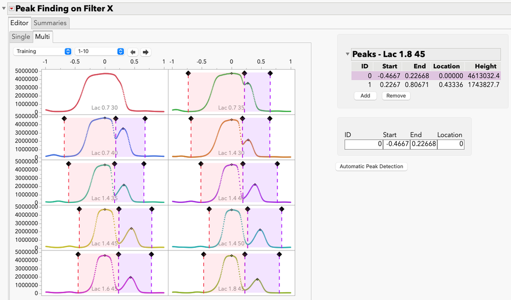
The end result
For this particular analysis, the end result of using Peak Finding is in the screenshot above. It took a few seconds for me to get to this point. I removed all the unwanted minor peaks. I also removed both peaks from the chromatogram in the upper left, because the two peaks were so bunched up against one another that we don’t (yet) have the tools to see where one starts and the other ends.
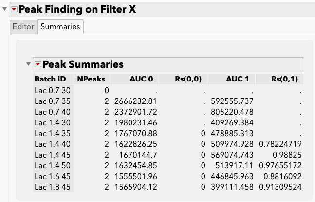
Under the Summaries Tab, we see things like the AUCs for the two peaks and their resolutions for each of the samples. Additional summary measures are available under the red triangle (under Customize Function Summaries).
From here, we can save the summaries to the data table and then model them using other tools in JMP.
What’s next for Peak Finding?
In the summary table above, we see that some of the resolutions (column Rs(0,1)) are missing. This is because we are using the U.S. Pharmacopeia definition of peak resolution, which is undefined when peaks are so poorly resolved that we don’t observe the location where the peak is at half of its overall height.
This brings me to a topic I am very excited about in the future for JMP Pro: Adding the capability to fit nonlinear regression models based on a sum of Gaussian peaks to the data. This capability will enable JMP Pro users to get a lot more out of their data in situations like you see here, ones with very poorly resolved peaks whose data we currently need to simply toss out like it never happened.