New features in Process Screening for JMP 16

[#1]

Process Screening enables you to explore a large number of processes across time. Several new features were added to this platform in JMP 16. This blog post details the new features for Process Screening that were introduced in JMP 16.

XBar and IMR charts in a single launch

Companies often have many ongoing processes. Some processes have more than one observation per subgroup and require an XBar chart, while other processes may have a single observation per subgroup and require an IMR chart. Beginning with JMP 16, you can get both chart types with a single Process Screening launch.

Consider the following data table.

dt=New Table( "Process Data",
	Add Rows( 24 ),
	New Column(
		"wafer", 
		Numeric( 1 ),
		"Nominal",
		Set Values(
			[1, 2, 3, 4, 5, 6, 7, 8, 9, 10, 11, 12, 1, 2, 3, 4, 5, 6, 7, 8, 9, 10,
			11, 12]
		),
		Set Display Width( 0 )
	),
	New Column(
		"Y1", 
		Numeric,
		"Continuous",
		Format( "Best", 10 ),
		Set Property(
			"Spec Limits",
			{LSL( 104.41 ), USL( 131.89 ), Target( 118.15 )}
		),
		Set Values(
			[114.555760105678, 113.52359591958, 114.946183872216, 116.25374611217,
			110.287898508744, 119.847995090729, 113.877878795723, 113.106755626713,
			114.832071507276, 115.737338527253, 120.193341974807, 113.425287275443,
			., ., ., ., ., ., ., ., ., ., ., .]
		),
		Set Display Width( 0 )
	),
	New Column(
		"Y2",
		Numeric,
		"Continuous",
		Format( "Best", 10 ),
		Set Property(
			"Spec Limits",
			{LSL( 164.39 ), USL( 429.65 ), Target( 297.02 )}
		),
		Set Values(
			[322.616751775796, 323.833298568833, 301.607366273833, 278.646245766939,
			469.298298488357, 332.715779503856, 346.462173291699, 213.59945858556,
			291.464226219377, 345.449129206092, 242.233144838257, 423.564714196848,
			291.370833295888, 333.921504947116, 288.644927205998, 258.806219486679,
			263.935377860945, 276.312880747942, 322.144968498633, 341.978235063698,
			316.143895248667, 302.164492808713, 319.751938178979, 269.802897971304]
		),
		Set Display Width( 0 )
	),
	Group Columns( "Processes", :Y1, 2 )
);  

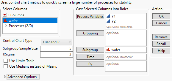
This table contains data from two processes. The first process (Y1) has one observation per wafer. The second process (Y2) has two observations per wafer. Therefore, the control chart type should be XBar for Y2 and IMR (Individual and Moving Range) for Y1.

To create this analysis, select Analyze->Screening->Process Screening. Assign Y1 and Y2 to Process Variables. Assign wafer to Subgroup. Change the chart type to XBar and R.

Alternatively, you can run the following JSL:

obj=dt<< Process Screening(
	Process Variables( :Y1, :Y2 ),
	Control Chart Type( "XBar and R" ),
	Subgroup( :wafer )
);

After clicking OK, you will find the following analysis:

An XBar and R chart type was applied to Y2. An Individual Measurement and Moving Range chart type was applied to Y1.

Color Out of Spec Values

Process Capability and Manage Spec Limits already provided methods to color values that are out of the specification limits.  This functionality was added to Process Screening JMP 16.

Run the following code to open Semiconductor Capability.jmp and run the Process Screening script attached to the table.

dt=Open("$SAMPLE_DATA/Semiconductor Capability.jmp");
obj=dt<<Run Script("Process Screening");

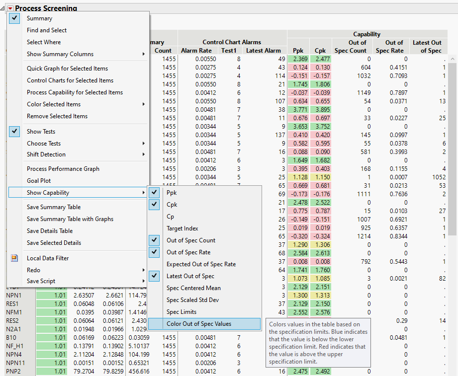
To color the out of spec values in your data table, select the red triangle next to Process Screening and choose Show Capability->Color Out of Spec Values.

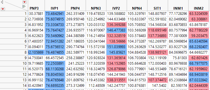
In the data table, cells with observations that fall below the lower spec limit are colored red. Cells with observations above the upper specification limit are colored blue.

Ability to specify K for K Sigma

Process monitoring is often plagued by too many false alarms. This can lead to the alarms being ignored. The K Sigma option, introduced in JMP 16, gives users the ability to specify K. Recall the limits are calculated using +/- K * Sigma, and increasing K will widen the limits. This gives you a way of making alarms less sensitive, producing fewer false alarms.

As an example, run the following:

dt=Open("$SAMPLE_DATA/Semiconductor Capability.jmp");
obj=dt<<Process Screening(
	Process Variables( :A2P1 ),
	Control Chart Type( "Indiv and MR" ),
	Subgroup( :Wafer ID in lot ID )
);

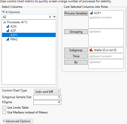
Note that there are 9 Test 1 violations. After investigations, it was determined that these were all false alarms. To make the alarms less sensitive, K Sigma can be adjusted. Select Analyze->Screening->Process Screening. Select A2P1 as Process Variables. Select Wafer ID in lot ID as Subgrouping.  In the bottom left of the dialog, change KSigma to 4.

Click OK.

A KSigma of 4 causes the control limits to be wider (center line +/- 4*sigma) as compared to a KSigma of 3 (center line +/- 3*sigma).  This example now has no test 1 violations as all observations fall within the 4 sigma limits.

Three key new features were added to Process Screening in JMP 16.

1. The ability to have XBar and IMR control charts in a single launch.
2. The ability to color and select out of spec values.
3. The ability to alter KSigma to make alarm tests more or less sensitive.