JMPer Cable
A technical blog for JMP users of all levels, full of how-to's, tips and tricks, and detailed information on JMP features- JMP User Community
- :
- Blogs
- :
- JMPer Cable
- :
- Minimize and Maximize Functions in JSL
- Subscribe to RSS Feed
- Mark as New
- Mark as Read
- Bookmark
- Subscribe
- Printer Friendly Page
- Report Inappropriate Content
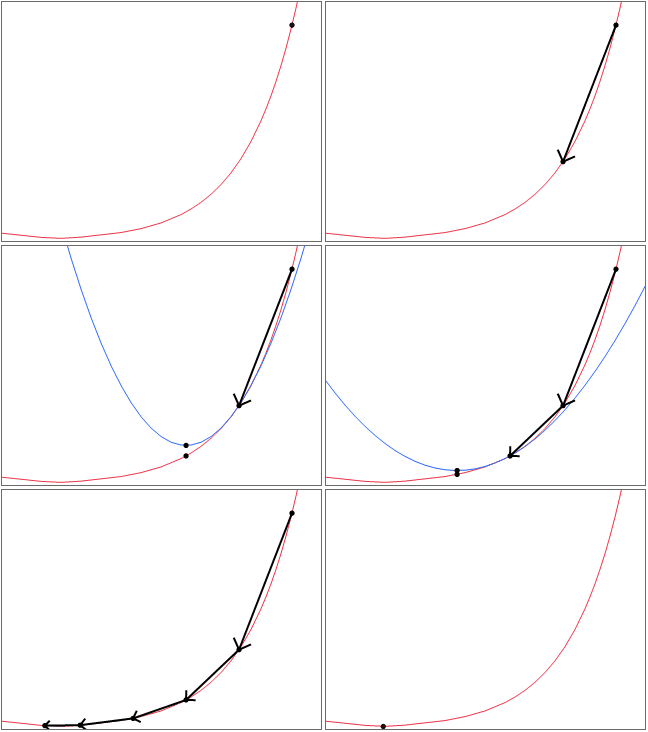
Among the many new features of JMP 13 are revamped Minimize() and Maximize() functions in JSL. These JSL functions are iterative optimizers that find the extreme values of a function given starting values. The GIF below a visual demonstration to give intuition for how the algorithm works in a simple one-dimensional setting.
While most JMP users will find pre-built platforms (such as Fit Y by X and Nonlinear) to be sufficient for their optimization problems, this isn’t always the case, and these JSL functions offer great flexibility and generality. These functions gives the user access to the same optimizers that JMP developers take advantage of when they are creating JMP platforms.
Generally speaking, anywhere that there is a likelihood reported in JMP, the model has been fit with an optimization technique called Maximium Likelihood. Similarly, the name, Least Squares, itself describes the optimization method used to fit linear models. While JMP has a wide variety of models available, there are times when one wants to fit a custom model that is not pre-built in JMP. Also, for pedagogical reasons, it can be useful for students to turn statistical modeling programs into optimization problems to understand how the model works.
The next few sections illustrate the basics of using a general optimizer. Users already familiar with iterative optimizers may want to skip to the last section to see example syntax for some of the advanced features in Minimize() and Maximize().
For the remainder of this article, I’ll write everything from the perspective of Minimize(). Note that minimizing a function, f(x), is equivalent to maximizing -1 * f(x), so exchanging “f(x)” with “–f(x)”, “minimize” with “maximize”, “concave” with “convex”, etc., will generalize the results to Maximize().
Simple Example
The most basic optimization problem requires two function arguments: an expression and the variables to optimize. As in the past, a call such as Minimize(expr, {x, y}) returns the minimum value obtained. To demonstrate how it works, the first example minimizes a trivial quadratic expression.
x = 2; /*starting value for x */
y = 2; /*starting value for y */
expr1 = expr((x ^ 2 + (y - 1) ^ 2));
minFun = Minimize( expr1, {x, y});
Show(minFun, x, y);
Output:
minFun = 0;
x = 0;
y = 1;
After some thought, we can convince ourselves that minimum of this function should be 0, and occur at x = 0 and y = 1. After running this script, we see that’s indeed the case.
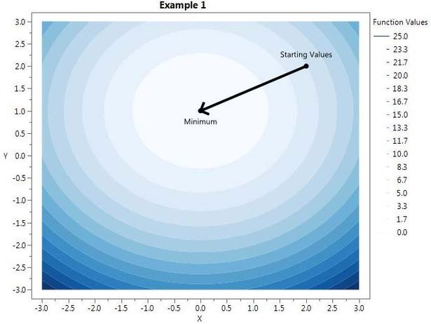
Notice that x and y have been changed by the Minimize() function to reflect the argument values that achieved the minimum function value. A contour plot for this function is shown here:
Choosing Starting Values
The optimizer has to begin with a particular set of parameter values, called starting values, and then iteratively tries to improve upon them. The success and failure of the optimization is highly dependent on the quality of the starting values. Part of the art of developing statistical software revolves around finding effective starting values. There are a variety of ways to come up with them. It is essential that the function can be evaluated at the starting values (i.e. it doesn't return a missing value). Sometimes the best you can do is come up with sensible ‘default’ values that work well, such as setting regression parameters equal to zero. Often the best starting values are obtained by fitting a simpler model to the data and using those results, such as using linear least squares estimates as starting values for a logistic regression.
Global vs. Local Critical Points
An important caveat to be aware of is that Minimize finds local critical points, which may or may not be the global minimum. The next example is a simple polynomial that illustrates this. With the starting values of x = 0, y = 0, a local minimum is found at x = 0.25, and y = -0.0833. However, for x=-1, and y = -1, the answer goes to –infinity.
x = 0; /*starting value for x */
y = 0; /*starting value for y */
expr2 = expr((y * 3 - 2 * x ^ 2 - 12 * x * y));
minFun = Minimize(expr2, {x, y});
Show( x, y, minFun);
Output:
x = 0.25;
y = -0.0833333333333333;
minFun = -0.125;
x = -1; /*starting value for x */
y = -1; /*starting value for y */
minFun = Minimize(expr2, {x, y});
Show( x, y, minFun);
Output:
Optimization failed: Failed: Maximum Iterations Exceeded

x = -6.55731043158825e+85;
y = -1.31136919553771e+89;
minFun = -1.03197258530774e+176;
Notice that Minimize() doesn’t give any warnings for this because it doesn’t know if it reached a local or a global minimum. In fact, in this example, the first set of starting values converge to a saddle point, which, in this case, is a minimum in one direction and a maximum in another. If a global minimum is desired, and the problem isn’t convex (or if you aren’t sure), then one option is to try multiple starting values to check if they all converge to the same location. Alternatively, if there are two or less parameters, the function can be plotted, which makes it easy to tell if it’s a local minimum, for example here is the countor plot from the last function with the two different starting values: 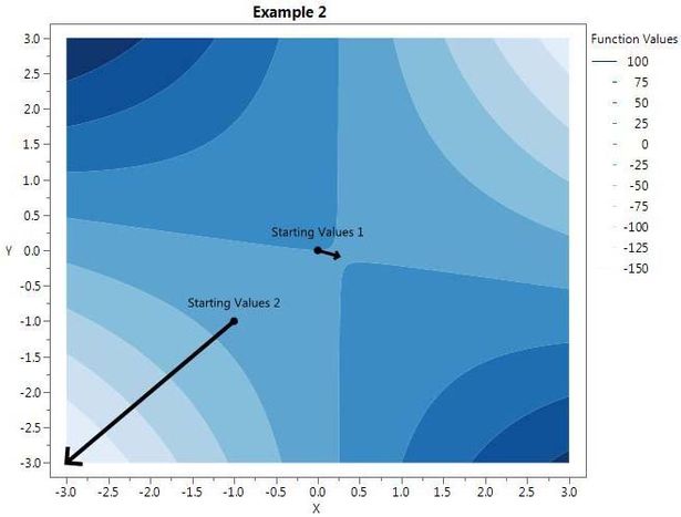
Realistic Example 1: Minimizing A Loss Function
In statistics, parameter estimates are often determined by finding the parameter values that minimize the sum of squared error terms, sum (observed – predicted) ^ 2. As an example, consider the Nonlinear NIST Dan Wood test case (“”).
Here, we want to minimize the sum of squared errors given the model, i.e. find the arguments for and
that minimizes
.
The following JSL code implements this.
x = [1.309, 1.471, 1.49, 1.565, 1.611, 1.68];
y = [2.138, 3.421, 3.597, 4.34, 4.882, 5.66];
b1 = 1; /*starting value for b1 */
b2 = 5; /*starting value for b2 */
sseExpr = Expr(
       Summation( i = 1, 6, (y[i] - b1 * x[i] ^ b2) ^ 2 )
);
minFun = Minimize( sseExpr, {b1, b2} );
Show( b1, b2, minFun );
Output:
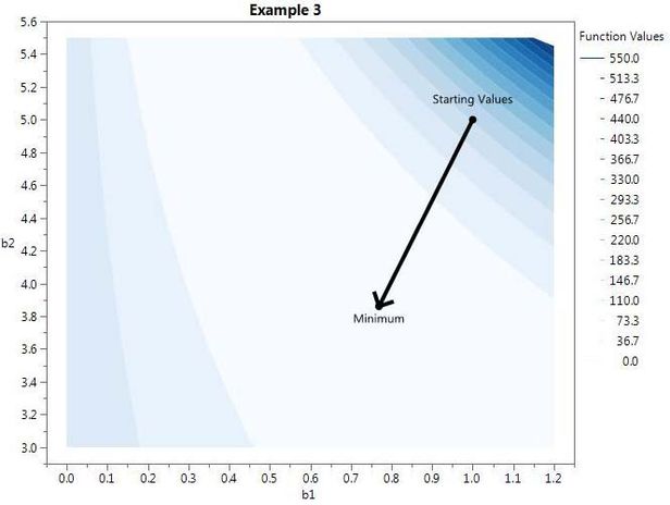
b1 = 0.768858626467797;
b2 = 3.86041439611906;
minFun = 0.00431730849313329;
Contour Plot:
Realistic Example 2: Simple Linear Logistic Regression
As mentioned, another common use of optimization routines is for finding maximum likelihood estimates. For example, say we have observed 100 binary response values, y, and an associated continuous predictor, x, and we want to fit a logistic regression model. For simple linear logistic regression, we assume that for each i, , where
. The associated log likelihood is
. For brevity, I skipped the derivations, but more details can be found here. The following JSL code maximizes this likelihood:
b0 = 0;
b1 = 0;
logLik = Expr(
       Summation( i = 1, 100, y[i] * log( logist(b0 + b1 * x[i]) ) + (1 - y[i]) * log(1- logist(b0 + b1 * x[i]) ) )
);
minFun = Maximize( logLik, {b0, b1} );
Show( b0, b1);
Output:
b0 = 0.169912186525928;
b1 = 2.37904556815702;
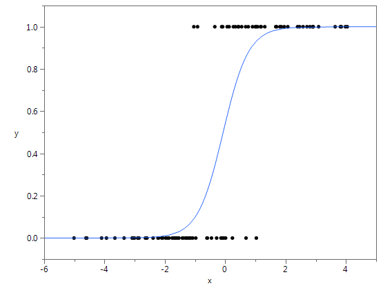
Thus, this model predicts that for some new x value, the estimated probabilities are:
With a plot of the fit:
If interested, please see the attached JSL script for the specific values of x and y that I used for this example as well as to see how I generated them.
New Optional Feature <<showdetails(true)
My favorite new feature allows the user to retrieve output details by using the optional argument <<showdetails(true). With this option selected, Minimize() shows the step-by-step results of the optimizer in the log. Additionally, instead of just returning the minimum function value, Minimize() returns a list with the following: minimum objective function value, number of iterations, gradient at the minimum, and hessian at the minimum. This is demonstrated on the NIST Dan Wood test case:
x = [1.309, 1.471, 1.49, 1.565, 1.611, 1.68];
y = [2.138, 3.421, 3.597, 4.34, 4.882, 5.66];
b1 = 1; /*starting value for b1 */
b2 = 5; /*starting value for b2 */
sseExpr = Expr(
       Summation( i = 1, 6, (y[i] - b1 * x[i] ^ b2) ^ 2 )
);
{objVal, iters, gradient, hessian} = Minimize( sseExpr, {b1, b2} , <<showdetails(true));
Show( b1, b2, objVal, iters, gradient, hessian );
Output:
nParm=2  Newton   ******************************************************

Iter   nFree   Objective  RelGrad    NormGrad2  Ridge   nObj   nGrad   nHess   Parm0      Parm1
0      2       149.7192   332.8046   182170.1   0       1      1       1       1          5
1      2       31.87877   101.5969   19003.84   0       1      1       1       1.010662   4.225573
2      2       4.215765   28.12531   1448.206   0       1      1       1       1.024865   3.630484
3      2       0.378951   7.636836   51.97781   0       1      1       1       1.058064   3.252922
4      2       0.153712   0.003012   0.615041   0.125   2      1       1       1.008287   3.272327
5      2       0.08553    0.100794   0.100071   0.031   1      1       1       0.937871   3.42031
6      2       0.035115   0.074061   0.132669   0.016   1      1       1       0.868411   3.588806
7      2       0.00829    0.164555   1.452852   0       1      1       1       0.772783   3.836035
8      2       0.00432    1.62e-5    0.00021    0       1      1       1       0.769751   3.858031
9      2       0.004317   2.313e-9   2.057e-8   0       1      1       1       0.768859   3.860414
Convergence SUCCESS: Gradient
Time: 0.033333333209157

b1 = 0.768858626467797;
b2 = 3.86041439611906;
objVal = 0.00431730849313329;
iters = 9;
gradient = [-0.000193577585687388, -0.000060622489899298];
hessian = [351.567213300015 123.108731500088, 123.108731500088 43.9222933905666];
List of All Optional Features for Minimize() and Maximize()
- Set Upper and Lower Bounds: Set lower and/or upper limits for variables. For example, Minimize( x^2, x(1,5) ), restricts x to stay between 1 and 5, and Minimize ( x^2, x(. , 5) ), ensures x is less than 5 with no lower bound.
- Set Maximum Number of Iterations: The maximum number of iterations defaults to 250 but can be changed with <<maxIter(newMaxIter). Defaults to 250.
- Set Tolerance for Convergence: The convergence criterion can be changed with <<tolerance(newTolerance). The default is 10^-8.
- Show More Details: The option <<showdetails(true), offers a variety of diagnostic tools for the optimizers. It is explained in more detail in the next section.
- Use Numerical Approximation for Derivatives: By default, Minimize() will attempt to find analytical derivatives, but in some cases, numerical approximations may work better. Select this option by adding "<<UseNumericDeriv(true)" to the function call. See an example at the bottom of this article.
- Input User-Defined Gradient: Most of the time, Minimize() will be able to calculate the analytical gradients by default. In the unlikely event that it's desired, a user can input their own gradient. To do this, use <<gradient(list of expressions), i.e. <<gradient({ d/dx1 (expr), d/dx2 (expr), ... } ). For an example, see the section below titled "Simple Example With All Optional Arguments."
- Input User-Defined Hessian: Inputting a user-defined hessian is even more cumbersome. The syntax gets complicated very quickly, and I'd recommend using this only as a last resort. To input an analytical hessian, use <<hessian (list of lists of expressions), with only the upper triangular portion of the hessian in row-major order. More specifically, this looks like: <<hessian({ {d^2/dx1^2 (expr), d^2/(dx1dx2) (expr), ... }, {d^2/dx2^2 (expr), ... }, ... } ). See example below.
Simple Example With All Optional Arguments
Below is a useful template of Minimize() with all the optional arguments selected. In JMP 13.2, this example can also be found under Minimize in the Scripting Index with JMP. It’s Example 3 (select it by choosing the drop down menu next to Example 1).
x = 0;
y = 0;
{objVal, iters, gradient, hessian} =
Minimize(
 ((2 * x ^ 2 + 12 * x * y - y * 3)),
 {x( -1, 1 ), y( -1, 1 )},
 <<maxIter( 200 ),
 <<tolerance( 10 ^ -6 ),
 <<ShowDetails( True ),
 //<<UseNumericDeriv( True ), /*rarely needed*/
 //<<Gradient({4*x+12*y, 12*x-3}), /*rarely needed*/
 //<<Hessian({{4,12},{0}}) /*rarely needed*/
);
Show( x, y, objVal, iters, gradient, hessian );
Stay posted for a possible future blog post on the new JSL functions, Constrained Minimize() and Constrained Maximize(), which optimize problems with nonlinear objective functions and linear constraints.
You must be a registered user to add a comment. If you've already registered, sign in. Otherwise, register and sign in.
- © 2026 JMP Statistical Discovery LLC. All Rights Reserved.
- Terms of Use
- Privacy Statement
- Contact Us

