In component reliability, or non-repairable system reliability, we assume that after a component has failed, it is discarded and can’t be repaired. Lifetime of components is modeled using Weibull or lognormal distributions (among others), and the goal is to estimate the time that a given proportion of parts will have failed or the proportion of parts that will fail at a given time.
In system reliability, or repairable system reliability, after the system has failed, it can be repaired by replacing non-repairable components with new ones. System reliability analysis is concerned with modeling the failures of systems of non-repairable components. The data come from a counting process – the response is the number of repair events at a given time. The goal is to model the mean cumulative function C(t), which gives the total number of events through time t. From this estimate, we can estimate the Intensity function I(t), which gives the repair rate.
Analysis of system reliability
If the distribution of failures has no memory, that is, the time between failures follows an exponential distribution, then the mean time between failures (MTBF) completely characterizes the process. However, if the time between failures follows a different distribution, then mean is changing over time and MTBF does not characterize the process adequately.
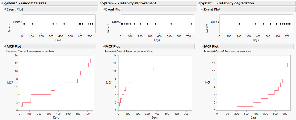
Graphical analysis, like the Event plot and the plot of the Mean Cumulative Function (Figure 1), can be used to determine if the repair rate is changing over time. Statistical models can be fit to describe the time between failures. The parameters of the model can be treated as functions of grouping variables or covariates.

Figure 1. Event plot and Mean Cumulative Function plot for three systems: one with random failures, one with improving reliability, and one with degrading reliability.
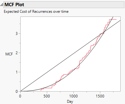
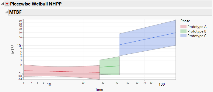
Models in the Recurrence platform include the homogeneous Poisson process and nonhomogeneous Poisson processes. Each model specifies the form of the mean cumulative function to be linear, polynomial, or exponential (Figure 2). The Reliability Growth platform allows you to model changes in reliability, either reliability improvement or degradation (Figure 3).

Figure 2. MCF plot for degrading reliability with models of the homogeneous Poisson process (linear) and power nonhomogeneous Poisson process (polynomial) added.

Figure 3. MTBF plot for reliability growth as modeled by a piecewise Weibull nonhomogeneous Poisson process.
Take a deeper dive into the reliability of repairable systems
View this series of short videos to understand how to visualize, describe, and make inferences about system reliability.
You must be a registered user to add a comment. If you've already registered, sign in. Otherwise, register and sign in.