One issue in data mining and statistics is collecting data and manipulating it into your software. Fortunately, JMP makes this very easy.
However, once you have the data, what do you need to do? First, you need to examine what you collected and "wrangle" the data (cleaning it, for instance) and then you need to analyze it. In this blog post, we'll examine all three areas: web data collection, data wrangling, and analysis.
Data Collection
Recent news has focused on various aspects of immigration into the United States. So let's explore trends in immigration to the US, specifically examining the number of persons obtaining lawful permanent resident status, "Green Cards." The relevant data is available for free from the US government in the 2016 Yearbook of Immigration Statistics. The specific webpage we'll extract data from is this:
https://www.dhs.gov/immigration-statistics/yearbook/2016/table1
This table has two columns of information: Year and Number, as seen below. This data is personally meaningful to me since my wife was one of these persons adding to the 2014 count. Without her, the count would have been 1,016,517 in 2014.
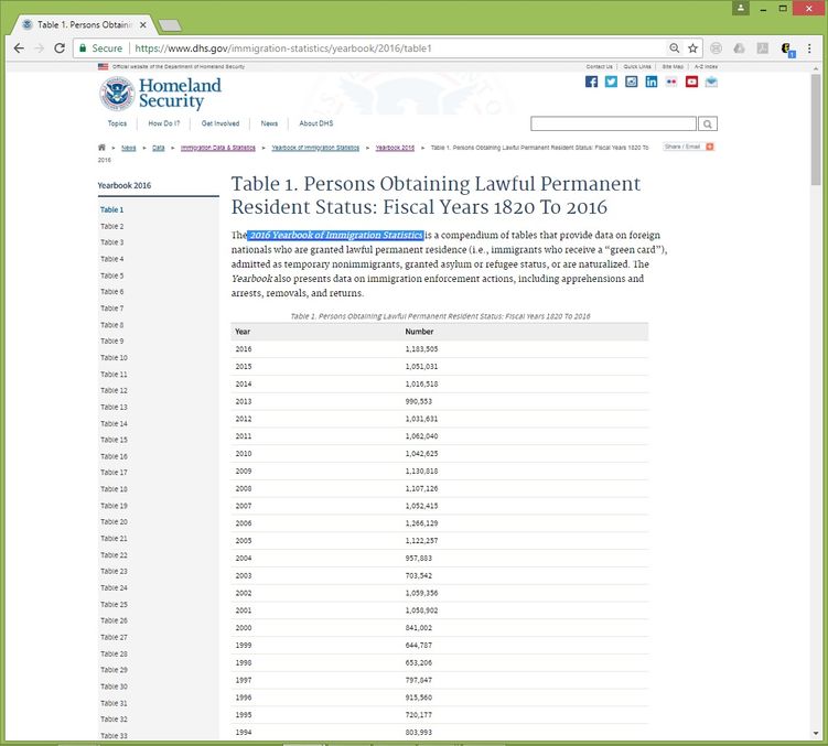 Table 1: 2016 Yearbook of Immigration Statistics
Web Data Extraction
Now that we have the target webpage to analyze, we need to get the data into JMP. For this, we can use Internet Open. This is a powerful tool, which can be found by going to File > Internet Open. From there, we see the following function (with the URL of interest already pasted). We have a few choices in how to open the webpage in JMP. For this example, we'll open the webpage as data and hope that the two columns of data are detected appropriately, which relies on the webpage developers organizing things logically. Once we have the URL pasted and select how to open the URL, we can click OK.
 Internet Open dialog box in JMP
Next, JMP will search through the webpage looking for tables that possibly contain data. What JMP has detected will be displayed to us in a list form. Luckily, this webpage had only one item that JMP believed was data. We need to select the table(s) we wish to open, Table 1 here, and then click OK.
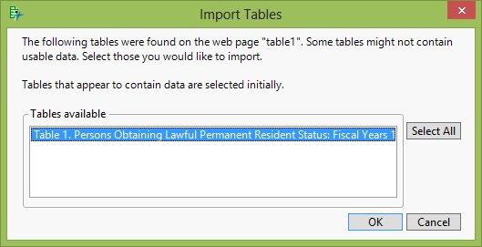 Importing Detected Tables
JMP will now create a new data table that contains the web-scraped data.
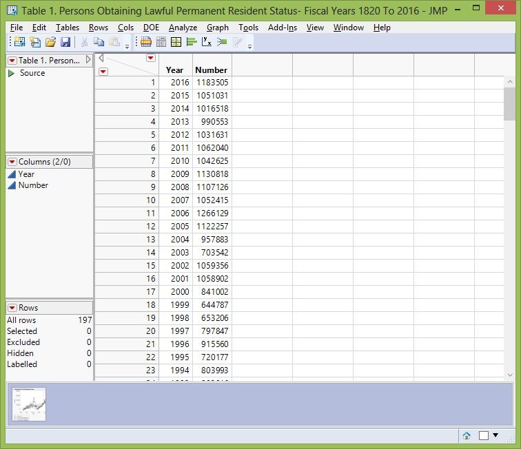 Resultant Data Table
Data Wrangling
At first glance, the data appears to have loaded effectively -- for example both variables are continuous (as we would expect), and glancing at the data shows nothing out of the ordinary. However, if we plot the data (using Graph Builder for instance), we see that we have an outlier at the year 1976.
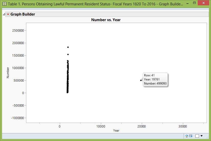 Data wrangling reveals an outlier
Apparently, 1976 was entered as 19761. So we must consider a few possibilities:
- Did someone "fat finger" 19761 and add an extra "1" to this year?
- Does the "1" go with the second column of data, i.e., making it 1,499,093 persons in 1976?
- Is it something else?
If we return to the original webpage, we see the third option is the right answer. The extra "1" was from a footnote that got transcribed by JMP as part of the year. The footnote presents information to the reader on the fiscal year change that occurred in 1976. For the sake of this analysis, we will remove the "1" only; however, a more thorough analysis might look at whether this accidentally over-counts in adjacent years.
I should make a further point for researcher: It's relatively easy to fix this problem since we naturally understand years. However, if a similar issue existed in the immigration data, we might be not able to detect it since this varies heavily. Thus, if you're creating data tables for the internet, think of future researchers and please put your footnotes in the most intuitive columns.
Data Analysis and Interpretation
For a quick analysis, we will use Fit Y by X and create various models. We can create more than just simple linear regression models in Fit Y by X, as discussed in Chapter 9 of my book Biostatistics Using JMP.
First we will fit a first order linear fit, i.e., linear regression, by selected Fit Line. This line, the red line below, is obviously not a good model for our data. Thus, we will proceed to create various higher-order polynomial fits, second through sixth order, as seen below.
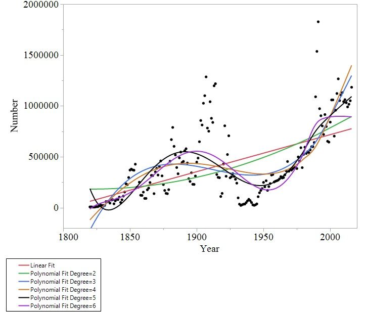 Applying Various Curve Fits
Visually, we can see that the second order fit (green line) doesn't appear to model the data well either. However, the third through sixth order fits appear to be capturing some of the complexities in the raw data. To me, the sixth order fit looks the best since it doesn't have the seemingly exponential increase around the year 2017 that we see in the third and fourth order fits. While the fifth order fit looks decent at the end of the data, it has an odd start. Thus, the sixth order model looks the best out of these options.
From here, we would want to examine residuals, etc. A rough analysis by examining variance explained can also help. The following table provides a rough assessment of quality of models via R-squared and R-squared adjusted. R-squared adjusted is important since it penalizes us for adding additional variables. Overall, the assessment shows that the sixth order model explains a lot of variation. Coupling that with our visual assessment of the models, the sixth order fit appears to be the best model created using this approach.
| Order |
R squared |
R squared adjusted |
| 1 |
0.336 |
0.333 |
| 2 |
0.359 |
0.353 |
| 3 |
0.552 |
0.545 |
| 4 |
0.562 |
0.553 |
| 5 |
0.639 |
0.630 |
| 6 |
0.669 |
0.659 |
Now this interpretation is with respect to the mean squares for a problem that has a lot of degrees of freedom allocated to error. So, the quality of any predictions from it any of these models could be low.
The next step might be to further explore the time series modeling capabilities in JMP using this data. However, this is enough for one day!
For more information on collecting data, including from the web, take a look at Chapter 2 of my book Biostatistics Using JMP. Chapter 3 of the book covers data wrangling in depth.
You must be a registered user to add a comment. If you've already registered, sign in. Otherwise, register and sign in.