- New to JMP? Let the Data Analysis Director guide you through selecting an analysis task, an analysis goal, and a data type. Available now in the JMP Marketplace!
- See how to install JMP Marketplace extensions to customize and enhance JMP.
- Subscribe to RSS Feed
- Bookmark
- Subscribe
- Printer Friendly Page
- Report Inappropriate Content
JMP Knowledge Base
- JMP User Community
- :
- Support
- :
- JMP Knowledge Base
- :
- Analyzing Repeated Measures in JMP® Software
Analyzing Repeated Measures Data in JMP® Software
Often in an experiment, more than one measure is taken on the same subject or experimental unit. This means that a repeated measures analysis of the data may be necessary to make valid inferences and to draw meaningful conclusions.
JMP offers multiple methods to analyze repeated measures: a multivariate repeated-measures approach, a univariate split-plot approach, and an additional capability through JMP® Pro to perform such an analysis with the Mixed Model personality within the Fit Model platform. The types of analyses are compared in the following discussion. The example uses the DOGS (dogs.jmp) sample data table, which is the result of a study with repeated measures. In this example, before performing analysis on the DOGS dataset, we will rename the ID variable as Subject and change the modeling type from continuous to nominal.
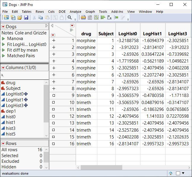
Figure A shows selected columns from the DOGS table. This data table contains information on sixteen dogs assigned to treatment groups defined by the independent variable drug, having values ‘morphine’ and ‘trimeth.’ The blood concentration of histamine is recorded before drug injection and again at one and three minutes after injection. The log of each value is taken (a common transformation to achieve more linearity in the response variable) which results in three variables, LogHist0, LogHist1, and LogHist3. Also, there is an additional Subject column, declared as Nominal as mentioned above, which will be used to account for the within-subject variability in a univariate analysis of repeated-measures data.
Figure A: Arrangement of Data Table, Multivariate Approach
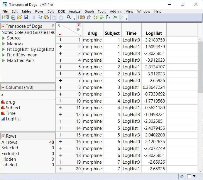
Figure B shows selected columns from the restructured DOGS table where the LogHist columns have been stacked into a single response column.
Figure B: Arrangement of Data Table, Univariate Split-Plot Approach and Mixed Model Approach
A Multivariate Approach
The original DOGS table with multiple response columns is in the form needed for a multivariate analysis of variance (MANOVA) that tests the same effects − nothing needs to be changed.
With this data table active, again choose Fit Model from the Analyze Menu.
Specify LogHist0, LogHist1 and LogHist3 as Y variables. Change the Fitting Personality to Manova. Assign drug as the model effect and run the model.
When there are multiple Y variables, JMP automatically performs a multivariate analysis. When you first run the model, the multivariate control panel appears. To test the effect of drug over time, select ‘Repeated Measures’ as the response design from the popup menu on the control panel. In the repeated-measures dialog that appears, use the default effect name Time but check ‘Univariate Tests Also’ to obtain univariate and adjusted univariate tests. This option includes a test of sphericity (not shown here), which checks whether the unadjusted univariate F tests are appropriate. If the sphericity chi-square test is not significant, you can use the unadjusted univariate F tests. However, if the sphericity test chi-square is significant, then the criterion is rejected and the multivariate F tests or the adjusted univariate F tests should be used. JMP gives both the Greenhouse-Geisser (G-G), and the Huynh-Feldt (H-F) adjusted F tests.
A Univariate Split-Plot Approach
A univariate model has a single response. To analyze the data as a univariate analysis of variance (ANOVA), you must include each source of variation (between-subjects and within-subjects) as an effect in the model.
The univariate analysis requires that the response measurements be in a single column. Using the Stack command in the Tables menu, you can stack the LogHist0, LogHist1 and LogHist3 columns to create a new response column, as shown in Figure B. The new response LogHist and the new classification variable Time were created by the Stack command.
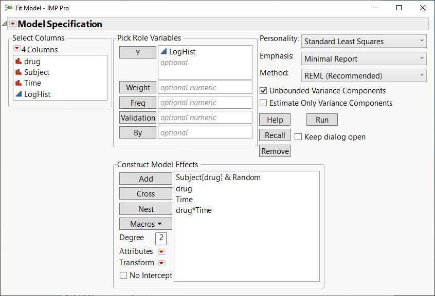
With the data table correctly set up, choose Fit Model from the Analyze Menu. Select LogHist as Y, and add the Effects in Model as shown in Figure C.
Figure C: Univariate Repeated Measures Specification
To create the model shown above, which has a random effect for testing the between-subjects effect in the model, click the following variables and buttons:
- drug in the variable selection list, then Add
- Subject in the variable selection list, then Add
- drug in the variable selection list, and
- Subject in the Effects in Model list, then Nest
- Subject [drug] in the Effects in Model list, then select Random from the Effect Attributes pop-up menu giving Subject [drug]& Random in the Effects in Model list
- Time in the variable selection list, then Add
- drug in the variable selection list and
- Time in the variable selection list, then Cross
The between-subject effect, drug, is the whole plot effect of a split-plot design. The Subject effect is nested within drug. This term is specified as a random effect. Random effects included in the model indicate multiple sources of variation in the data. All sources of variation are taken into consideration in the REML model; therefore effect estimates and effect tests are adjusted and calculated appropriately.
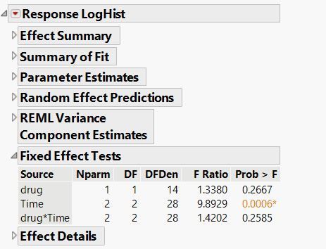
After running this model you can examine the significance of the model effects seen in the ‘Fixed Effect Tests’ section in the results window, which are shown below in the Comparing Results section.
Mixed Model Approach
In JMP Pro, the Mixed Model personality within the Fit Model platform also offers the capability to analyze repeated measures data. This method requires the response measurements to be structured in a single column as displayed in Figure B.
The Mixed Model personality fits a variety of covariance structures. This is in contrast to both the MANOVA, which assumes an unstructured covariance matrix where all variances and covariances are estimated individually, and the univariate split-plot ANOVA, which assumes all errors are independent. When data is normally distributed, the latter is equivalent to assuming a compound symmetry covariance structure within a Mixed Model.
With the data table active, choose Fit Model from the Analyze Menu. From the Personality drop down menu, select Mixed Model. Assign LogHist as the Y variable, add Time, drug, and drug*Time in the Fixed Effects tab, and add Subject to the Random Effects tab. Click on the Repeated Structure tab and keep the default selection, ‘Residual’, which represents the compound symmetry covariance structure. In this example, we’ll use this option to show consistent results across method. As explained in the previous paragraph, the compound symmetry structure is equivalent to the assumed covariance structure in a univariate split-plot analysis.
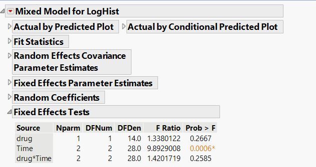
Run the model and the significance of the fixed effects will appear in the last section of the results window.
Comparing the Results
Multivariate Approach
Univariate Split Plot Approach
Mixed Model Approach (JMP Pro only)
Comparing the Methods
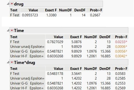
A comparison of analysis results is shown above. By examining each set of results, you can see the relationship among the multivariate and univariate effects tests, including the mixed model analysis. Important points to note are:
- For between-subject effects (drug), the multivariate approach gives the same results as the univariate approach when there are no missing values. If there are missing values, a univariate analysis uses all non-missing data values but the multivariate analysis excludes any subject with any missing values.
- If there are no missing values, the within-subjects Time variable in the univariate model is the same as the unadjusted Time effect in a multivariate model having a ‘Repeated Measures’ response design. However, these tests are appropriate only if the sphericity test criterion (mentioned previously) is met. Otherwise, the multivariate tests or the adjusted univariate tests should be used.
- Using the compound symmetry covariance structure within the Mixed Model personality generates the same results as the univariate split-plot analysis because of the fairly normal distribution of the data. With data containing repeated measures in time, note that the alternative covariance structure AR(1) frequently is appropriate, as it allows for correlated observations but does not overfit the model.
- Often in a repeated-measures study the most important effect is the within-subject by between-subject interaction– the hypothesis of interest is whether the study treatment has an effect over time. In the univariate analysis, the drug*Time interaction appears insignificant.
- In this example the more powerful multivariate approach shows the drug*Time interaction effect to have marginal significance.
Summary
In summary, JMP can analyze repeated measures data with a univariate split-plot model, a multivariate analysis or, with JMP Pro, a mixed model.
Each type of analysis has its advantages and disadvantages:
- The multivariate analysis is easy and intuitive to specify in JMP. Its tests are usually more powerful. From a computing standpoint, this method is most efficient. However, if a subject is missing a value, all information for that subject is lost to the analysis.
- The univariate analysis can use all the data–only a subject's missing measurement is lost to the analysis. However, the univariate analysis can be very computationally intensive, particularly if there are many subjects.
- Both of the above methods assume an extreme covariance structure. The multivariate analysis assumes unstructured covariance matrix where all variances and covariances are estimated individually. The split-plot analysis assumes all errors are independent. With both of these assumptions, information in your data is used to estimate the covariance parameters. This can result in the overfitting of your model. The advantage of a mixed model is that it allows you to select a less extreme covariance structure resulting in a more powerful model. In the JMP Fitting Linear Models Guide, the Additional Examples section of the Mixed Models chapter offers more information about overfitting or underfitting a model and usage of the various covariance structures in the Mixed Model personality.
In the univariate tests for within-subject effects and interactions involving these effects, the above assumptions about the covariance matrix are required for the probabilities provided by the ordinary F tests to be correct. If these assumptions are not met (if the sphericity test is rejected), then probabilities for adjusted univariate F tests (given in the multivariate report) or the multivariate F tests should be used. Because of these assumptions, the univariate approach should be considered only when the Sphericity condition is met. For more information on this test and other ideas discussed in this sample, see the JMP Fitting Linear Models book, which is found by selecting Help ► Books ► Fitting Linear Models (Chapter 3: Standard Least Squares Report and Options, Chapter 7: Mixed Models, and Chapter 8: Multivariate Response Models)
Cole and Grizzle, J.E. (1966), "Sixteen Dogs," Biometrics, 22:810
[Previously JMP Note 30584]
Recommended Articles
- © 2026 JMP Statistical Discovery LLC. All Rights Reserved.
- Terms of Use
- Privacy Statement
- Contact Us
