 If you are experimenting without using DoE, you are almost certainly wasting your time. A real-world example with water testing data shows why.
I hate to see people wasting their time. That is why I never tire of telling scientists and engineers to use design of experiments (DoE). If they are experimenting without using DoE, they are almost certainly wasting their time.
DoE can appear almost magical at first sight. One person even told me that it is a religion! That made me laugh. Probably because I think there is a grain of truth in what that person said.
I want to demystify DoE with simple explanations of some of the terms and concepts that can be confusing for people when they are starting out. I hope that by walking through a case study, you will find that there are only compelling, rational reasons for statistically designed experiments. You don’t need to have blind faith.
In this first post about this topic, I want to immerse you in the overwhelming scale of the possibility space for multi-parameter processes and systems – and to show you how we can overcome the challenge with smart ways of exploring this space to learn the most we can with no wasted time or effort.
A real-world example
The example we have is from analytical method development. We want to develop the best method for measuring the concentration of organochloride pesticides and polychlorinated biphenyls (PCBs) in water. Measuring organic compounds in water is a routine, high-volume and high-throughput task for many environmental laboratories.
Labs need to optimise their analytical method in order to achieve the best limit of detection to meet legal requirements. The method also needs to be robust and provide consistent results. The analysis uses GC-MS: gas chromatography (GC) to separate the components in the sample and mass spectrometry (MS) for detection.
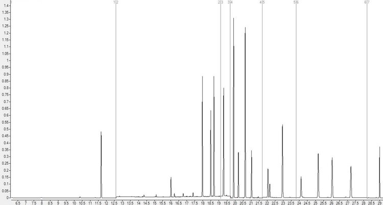 A typical chromatogram showing the peaks for each substance or analyte. Taller peaks correspond to a higher amount of that analyte. We want to find conditions that give us the tallest peaks for all analytes so that we can detect substances that are in water at very low concentrations.
A large volume injector (LVI) needs to be used to introduce the sample to the GC-MS system to enable detection of substances at very low concentrations. The challenge is that LVIs are complex, with many parameters that need to be optimised to find the best conditions. We are looking to find conditions that give the tallest peaks – the strongest signal – in the gas chromatogram.
Factors, runs and responses
There is nothing special here that means DoE is uniquely useful. DoE is useful in situations like this where you are searching to find the best settings of parameter combinations in a large space of possibilities. DoE is also useful when you need to know how to control the system or process by understanding all the important behaviours.
Let’s look at the possibilities for our LVI set-up. There are eight parameters that we can change:
| Factor |
Abrv. |
Lowest |
Highest |
| Injection Volume |
Vol(Inj) |
10µL |
100µL |
| Injection Speed |
Speed(Inj) |
0.25 µL/s |
5 µL/s |
| Injection T -30°C-30°C |
T(Inj) |
-30°C |
30°C |
| Injection Depth |
Depth(Inj) |
20mm |
40mm |
| Vent Flow |
Flow(Vent) |
10mL/min |
150 mL/min |
| Vent Pressure |
P(Vent) |
0psi |
9psi |
| Vent time |
t(Vent) |
0.1min |
1min |
| Liner type |
Liner |
Type1 |
Type2 |
In DoE, these are called the factors. For each of these factors, we also have a range of settings: the range over which we are going to experiment. The factors and their ranges define the possibility space within which we expect to find the solution. How are we going to explore the infinite possibilities?
To get an idea of the number of possibilities, we will constrain our search such that we will consider each factor at only three settings in the range: lowest, mid-point and highest (L, M, H). For example, we will only consider setting Injection Volume at 10, 55 or 100 µl. (There are good reasons why you would want to look at L, M and H settings for each factor, and we can talk about this in a later post.)
If we take just the first two factors and we wish to measure all combinations of L, M and H, we would have 3 * 3 = 9 different settings to test. We call these runs in DoE. We can visualise the possibility space and see the runs that we would carry out in a simple plot.
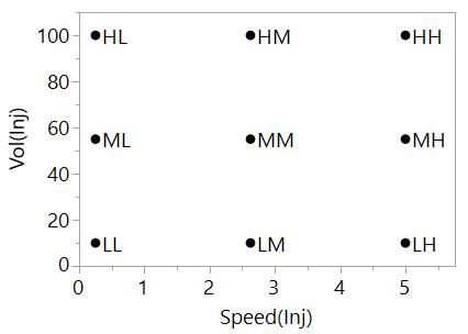
We call this type of experimental design a full factorial because we are testing the full set of factor combinations for the chosen number of levels. This full factorial will give good coverage of the possibility space. By running a standard sample through the system at these nine settings and measuring the peak height, our response, we will have useful information to find the settings of these factors that will maximise the response and our ability to detect substances at low concentrations.
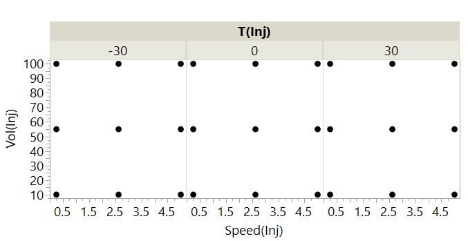
If we extend this to three factors, there are now 3 * 3 = 9 combinations for each of the three settings of T(inj) = 3 * 3 * 3 = 3^3 = 27 combinations. We begin to see the explosion of possibilities in multi-factor space.
To test every combination for our first seven factors at three levels, we would have 3^7 = 2187 possibilities!
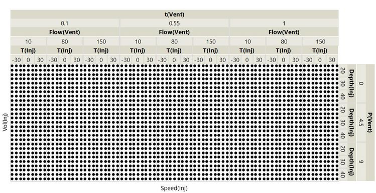
What about Liner type? That factor is different because it can only be Type1 or Type2. We say it is a categorical factor, whereas the others are continuous factors. We would test each of the 2187 combinations with the two different liner types, giving a total of 4374! You can count the dots if you don’t believe me.
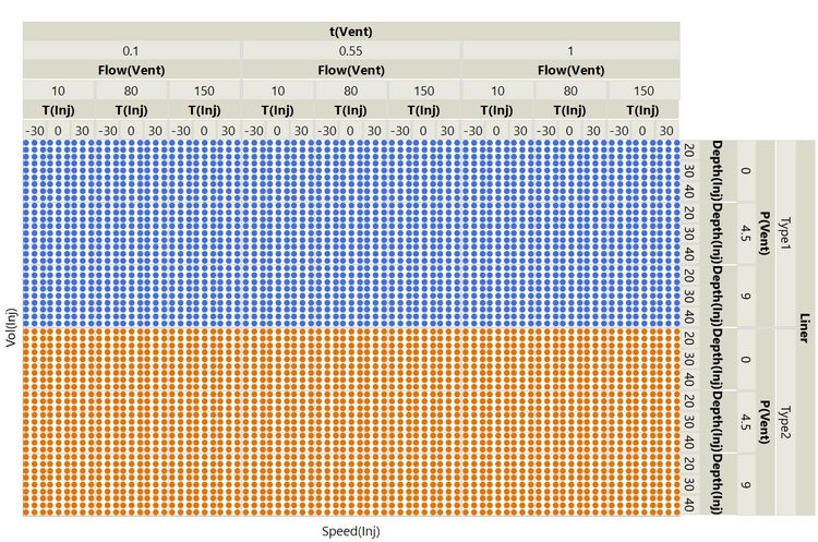
Don’t worry if you can’t make much sense of this plot. You can see it is difficult to visualise all these possibilities. I include it to give you a sense of the overwhelming number of possibilities. Unless you have a large team of minions, it will not be feasible to carry out this kind of experiment.
From 4374 runs to 26 runs
How are we going to find the best setting out of all of that? And how can we hope to understand the behaviour of the system at any point in the space? You can see how you could use up a lot of time trying different combinations without much chance of learning anything useful.
Do not despair: This is where the magic of DoE comes in. Instead of the full factorial of 4374 runs, we can take a smaller subset and gain much the same useful information.
These 26 runs would form a useful experiment for our objective:
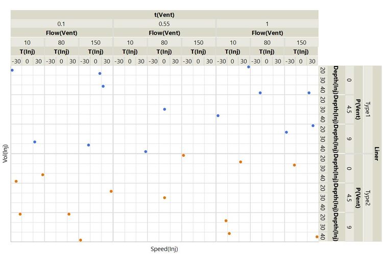
Why these 26 runs? Have they just been chosen at random? Some of you might have spotted that there is a certain symmetry, but otherwise it is not obvious why these runs should be selected. Also, what about the other 4348 runs? Don’t we need to worry about what might happen at those settings? And the settings in between?
In my next posts, I will answer these questions and use the example to visually illustrate key concepts in DoE.