- New to JMP? Let the Data Analysis Director guide you through selecting an analysis task, an analysis goal, and a data type. Available now in the JMP Marketplace!
- See how to install JMP Marketplace extensions to customize and enhance JMP.
JMP Blog
A blog for anyone curious about data visualization, design of experiments, statistics, predictive modeling, and more- JMP User Community
- :
- Blogs
- :
- JMP Blog
- :
- The QbD Column: Response surface methods and sequential exploration
- Subscribe to RSS Feed
- Mark as New
- Mark as Read
- Bookmark
- Subscribe
- Printer Friendly Page
- Report Inappropriate Content
Editor's note: This post is by @ronkenett, @david_s and Benny Yoskovich of the KPA Group. It is part of a series of blog posts called The QbD Column. For more information on the authors, click the authors' community names above.


George Box and K.B. Wilson introduced the idea of response surface methodology in a famous article[1] in 1951. There were several novel and extremely useful ideas in the article:
- Designed experiments can be a great tool in experimentally optimizing conditions.
- When feedback is rapid, there are great benefits to breaking up the experimental effort into a sequence of experiments, rather than trying to “learn everything at once”.
- The results of one experiment will often stimulate changes in strategy: new factors may be added, old ones may be dropped, factor ranges may move.
- The results may indicate that a more complex regression model is needed to adequately reflect the relationship between the factors and the outcomes.
A typical response surface study begins with a screening experiment to identify the most important factors. Small, orthogonal experimental plans and simple regression models are usually used for screening (see our second and third blog posts in this series). Subsequent experiments will depend on the results of the screening experiment. For example, factors that had small effects might be dropped from further consideration. Other factors might be added. The team might decide to shift the levels of some of the factors to get better results for the critical quality attributes (CQA’s). If the results suggest that a first-order model is no longer a good fit to the data, the team expands the design to permit fitting a second-degree regression model. Box and Wilson proposed the central composite design for that purpose, and to this day, it remains a popular choice.
How is response surface methodology used in QbD?
Many QbD studies are aimed at determining improved production conditions and are able to exploit the benefits of sequential experimentation. These studies can benefit from response surface methodology.
We illustrate the approach and some of the methods via a study reported by Xu, Khan and Burgess[2]. Their goal was to use designed experiments to improve the drug delivery system for a class of molecules by using liposome formulations. Such formulations were expected to bring benefits by improving the ability to target the activity of the molecule in the body. However, previous efforts had yielded methods that were not commercially viable, primarily because an important critical quality attribute (CQA), encapsulation efficiency, was too low.
The experimental team focused on three CQAs in this sequence of experiments: encapsulation efficiency (with a goal of at least 20%); particle size (with a target range of 100-200 nm); and storage stability at 4⁰ C. They also carried out a risk analysis to decide which process factors to study, converging on a list of eight: lipid concentration; drug concentration; extrusion pressure; cholesterol concentration; buffer concentration; hydration time; sonication time; and number of freeze-thaw cycles.
What design was used for factor screening?
The first experiment was aimed at finding the most important factors from the list of eight. The team wanted a small, economical experiment, and so chose to use a 12-run Plackett and Burman (PB) experiment. This is an orthogonal experiment that can screen up to 11 factors, each at two levels. Like most PB designs, the 12-run design does not completely alias two-factor interactions with main effects. Sometimes this has beneficial effects for screening, enabling detection of an especially large interaction when there are only two or three active factors. The team also added three center points, which enables a pure-error estimate of variability and a check on the need for pure quadratic terms.
It is easy to generate the PB design in JMP using the Screening Design platform within DOE. After entering the factors, check the box for choosing from a list of orthogonal designs and the 12-run PB design is at the top of the list, due to its economical run size. After selecting this design, there is an option to add center points.
The team looked at three immediate outcomes from the experiment: encapsulation efficiency (EE); particle size; and zeta potential. In addition, each formulation was diluted and divided into samples for storage, half at 4⁰ C and half at 37⁰ C. These samples were tested at predetermined times (up to 24 months) for loss of active drug during storage.
What were the results of the data analysis?
The 15 experimental runs had EEs that ranged from 8.2% to 36.5%. Figure 1 shows a summary of the data analysis for EE. Lipid concentration was clearly the most important factor – increasing the lipid concentration led to higher EE. Drug concentration was also highly significant, with a negative effect on EE. None of the other factors reached statistical significance, and all had effects that were quite small compared to those of the two strong factors. The fit to the data was very good. The residual standard deviation was 0.87% (quite small compared to the range of EE results), and there was no evidence of lack of fit.
Figure 1: Factor effects on EE in the initial PB experiment
The analysis of particle size focused on the mean particle size for each experimental run. These means were all between 160 and 176 nm, well within the acceptable range. None of the factors had strong effects on mean particle size, suggesting that this outcome is highly robust to the settings of the factors in the experiment. Particle size also varies within experimental runs, and the team measured the standard deviation. The SDs were all 3.1 nm or less, so that particle size was actually quite uniform within runs.
The zeta potential is a measure of the magnitude of the electrostatic or charge repulsion/attraction between particles, and known to affect stability. All the process runs in the PB design had zeta potential between 61 and 76. None of the factors had a statistically significant effect on the outcome.
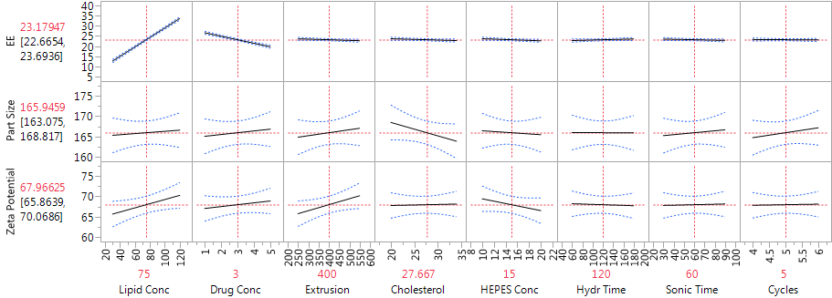
Figure 2 shows the JMP Profiler for the three immediate responses. The strong effects of lipid concentration and drug concentration on EE are evident in Figure 2, as are the weak effects of all the factors on both mean particle size and zeta potential.
The study team was also concerned about storage stability. They assessed stability by measuring drug leakage over a two-year storage period. For the samples stored at 4⁰ C, there was almost no leakage. So cold storage led to excellent stability regardless of the process factor settings. The samples stored at 37⁰ C did suffer from drug leakage, with an average loss of 6.6% after just two weeks of storage. Xu et al. did not present the data on leakage. The summary analysis in their article shows that the factor with the strongest effect on leakage was the lipid concentration; the high setting of 120 for this factor led to a decrease from 6.6% to 3.4%. The use of higher lipid concentrations was thus helpful both for increasing EE and for improving storage stability. The primary conclusions of the storage analysis were that it is important to store at cold temperatures and, when that is done, the drug remains stable for up to two years regardless of the factor settings.
Figure 2: Profiler showing the factor effects on EE, particle size and zeta potential, from the main effects model
Can we identify any interactions?
We pointed out earlier that one of the advantages of the PB design is that, when there are few active factors, it may be possible to identify an important two-factor interaction. One useful strategy is to look at all the interactions between two factors with active main effects, using stepwise regression to decide which interactions have the most predictive power. The drug delivery experiment found just two active factors, so the interaction between them is the only candidate. Figure 3 shows the results from fitting the corresponding model. The interaction is strongly significant, much more so than any of the other six main effects. This is a solid indication that there are second-order effects associated with the two dominant factors.
Note that the main effect estimates do not change from those in Figure 1 – this is because of the orthogonality of the Plackett-Burman design. When the design is projected onto two factors, as in this analysis, it has three replicates of each of the four combinations of those factors, so adding their interaction does not affect the orthogonality. However, when more factors and/or interactions are included, the model is no longer orthogonal, and the effect estimates will change.
Figure 3: Model for EE with main effects of lipid concentration, drug concentration and their interaction
How did the study proceed?
The initial experiment clearly pointed to lipid concentration and drug concentration as the two process factors that affect EE. The team decided to focus on these two parameters in the second phase of the study, holding all the other factors at default levels. They wanted to explore the possibility of curvature in the relationship, and so chose to use a central composite design (CCD), which allows fitting a full second-order model. The CCD has three types of experimental runs. One set is a two-level factorial. Another set consists of center points. The third set has “axial points,” in which one factor is set at two extreme levels and all the others are at their center settings. The extreme levels can be the same ones used for the factorial points (in which case the CCD has factors at three levels) or can be different (in which case the factors have five levels).
In the drug delivery study, the team used five levels for each factor. When five levels are used, the axial points are usually set to levels outside those for the factorial points. So it is also common to extend the ranges of the factors. The experimental range for lipid concentration was stretched upwards from that used in the PB experiment (30-160 instead of 30-120), and the range for drug concentration was extended in both directions (0.5-8 instead of 1-5). The experiment included 12 runs: four factorial points, four axial points (two for each factor) and four center points.
Other strategies can also be used to augment a screening design and fit a higher-order model. When there are more than two or three active factors, it is often possible to find expanded designs that are smaller, hence more economical, than the CCD. One useful option is to apply the custom design platform in JMP for a full quadratic model. The I-optimal design is a good choice here, with small run size and good ability to estimate the response function throughout the factor space.
What were the results of the CCD?
The results for EE in the second phase of the study were from 9% to 41%. The low EE occurred when the lipid concentration had its low value of 30, matching the findings from the initial experiment. The CCD is specifically designed to let us fit a full second-order model using a relatively small number of experimental runs. That model includes linear and quadratic main effects for each of the factors and all two-factor interactions. We used JMP to fit the second-order model to the data from the drug delivery system experiment via the Fit Model menu. To construct the model effects, choose the two experimental factors and then click on the Macros option and choose Response Surface. Figure 4 shows the results.
Figure 4: Second-order model fit to the CCD data
The two factors have strong linear effects, much as in the original screening experiment. The figures show scaled estimates and, because the factor ranges were wider in the CCD, the coefficients relate to the wider scale. The change in ranges results in larger coefficients in the CCD. Both factors also have significant pure quadratic effects. The interaction effect is similar in magnitude to that in the original experiment, but opposite in sign. Again, it is quite possible that this relates to the fact that the model is being fitted to a wider range in the factor space. The interaction effect does not achieve statistical significance here, and that is probably due to the small size of the factorial portion of the CCD. In this experiment, only four observations contribute to estimating the interaction; in the original PB experiment, all 12 observations were relevant.
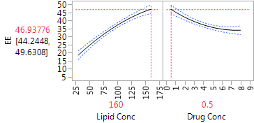
The Profiler (in Figure 5) is very helpful for “combining” the linear and quadratic effects of the two factors. We can see that for both factors, the dominant effect is the linear effect. The estimated effects are monotone throughout the region of experimentation. The Profiler has both factors set at their optimal settings, within the range of the experiment, with an estimated level of EE equal to 46.9. The quadratic effects suggest that the effects are stronger at low levels of each factor than at high levels. Hence, higher levels of lipid concentration might produce even higher EE, but the marginal benefit is decreasing. Lower drug concentrations also generated higher EE, and there the gain from further reduction could be substantial. Of course, we always need to be careful about extrapolating outside the experimental range, and any proposal to use more extreme settings should be tested in further experimentation.
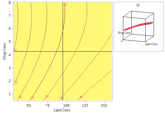
Figure 6 shows a contour plot of predicted EE levels based on the CCD. The highest predicted values are obtained with high lipid concentrations and low drug concentrations. Using high lipid concentrations gives good predicted values for the full range of drug concentrations that were included in the experiments.
Figure 5: Profiler plot for the CCD
Figure 6: Contour plot for predicted EE using the model from the CCD
How did the team verify the models?
To further test the validity of the model for predicting EE, the team ran a number of additional experiments, varying the settings of lipid concentration and drug concentration. For example, drug concentrations of 1% and 5% were matched with several lipid concentrations ranging from 30% to 150%. Some of these combinations are at the border of the region tested in the CCD. A number of other combinations within the domain of the CCD were also tested. The results showed excellent agreement between the new data and the predictions based on the CCD.
What did the team conclude?
The study team used the experiments to derive a design space for the specific active ingredient used in this project. They were convinced that the conclusions would be quite general and would prove relevant to many other hydrophilic agents. Thus, they saw these experiments as the springboard to developing effective procedures for many additional settings. The good results regarding storage at low temperature were also highly encouraging. They showed that the product could remain stable at low temperatures for up to two years, without the need to make adjustments that would complicate and add expense to the production process.
Next in this series
The next blog posts in this series will cover nonlinear designs, split plot design and robust designs, in the context of QbD.
References
[1] Box, G. and Wilson, K. (1951), On the Experimental Attainment of Optimum Conditions, Journal of the Royal Statistical Society. Series B (Methodological), Vol. 13, No. 1, pp. 1-45.
[2] Xu, X., Khan, M. and Burgess, D. (2012), A quality by design (QbD) case study on liposomes containing hydrophilic API: II. Screening of critical variables, and establishment of design space at laboratory scale, International Journal of Pharmaceutics, 423, pp. 543– 553.
- © 2026 JMP Statistical Discovery LLC. All Rights Reserved.
- Terms of Use
- Privacy Statement
- Contact Us


You must be a registered user to add a comment. If you've already registered, sign in. Otherwise, register and sign in.