- New to JMP? Let the Data Analysis Director guide you through selecting an analysis task, an analysis goal, and a data type. Available now in the JMP Marketplace!
- See how to install JMP Marketplace extensions to customize and enhance JMP.
JMP Blog
A blog for anyone curious about data visualization, design of experiments, statistics, predictive modeling, and more- JMP User Community
- :
- Blogs
- :
- JMP Blog
- :
- The QbD Column: Applying QbD to make analytic methods robust
- Subscribe to RSS Feed
- Mark as New
- Mark as Read
- Bookmark
- Subscribe
- Printer Friendly Page
- Report Inappropriate Content
Editor's note: This post is by @ronkenett and @david_s of the KPA Group. It is part of a series of posts called The QbD Column.
In our previous blog post, we wrote about using designed experiments to develop analytic methods. This post continues the discussion of analytic methods and shows how a new type of experimental design, the Definitive Screening Design[1] (DSD), can be used to assess and improve analytic methods.
We begin with a quick review of analytic methods and a brief summary of the experiment described in that previous blog post, and then show what is learned by using a DSD.
What are analytic methods?
Analytic methods are used to carry out essential product and process measurements. Such measurement systems are critical in the pharmaceutical industry where understanding of the process monitoring and control requirements are important for developing sound analytic methods. The typical requirements for evaluating analytic methods include:
- Precision: This requirement makes sure that method variability is only a small proportion of the specifications range (upper specification limit – lower specification limit).
- Selectivity: This determines which impurities to monitor at each production step and specifies design methods that adequately discriminate the relative proportions of each impurity.
- Sensitivity: This relates to the need for methods that accurately reflect changes in CQA's that are important relative to the specification limits, which is essential for effective process control.
QbD implementation in the development of analytic methods is typically a four-stage process addressing both design and control of the methods[2]. The stages are:
- Method Design Intent: Identify and specify the analytical method performance.
- Method Design Selection: Select the method work conditions to achieve the design intent.
- Method Control Definition: Establish and define appropriate controls for the components with the largest contributions to performance variability.
- Method Control Validation: Demonstrate acceptable method performance with robust and effective controls.
We continue here the discussion of how to use statistically designed experiments to achieve robustness, which we began in our previous blog post.
A case study in HPLC development
The case study we presented in our previous post concerns the development of a High Performance Liquid Chromatography (HPLC) method[3]. The specific system consists of an Agilent 1050, with a variable-wavelength UV detector and a model 3396-A integrator. Table 1 lists the factors and their levels used in the designed experiments of this case study. The original experimental array was a 27-4 Fractional Factorial experiment with three center points (see Table 2). The levels "-1" and "1" correspond to the lower and upper levels listed in Table 1, and "0" corresponds to the nominal level. The lower and upper levels are chosen to reflect variation that might naturally occur about the nominal setting during regular operation.
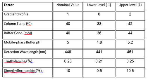
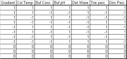
The fractional factorial experiment (Table 2) consists of 11 runs that combine the design factor levels in a balanced set of combinations, including three center points.
What do we learn from the fractional factorial experiment?
In our previous post, we analyzed the data from the factorial experiment and found that the experiment provided answers to several important questions:
- How sensitive is the method to natural variation in the input settings?
- Which inputs have the largest effect on the outputs from the method?
- Are there different inputs that dominate the sensitivity of different responses?
- Is the variation transmitted from factor variation large relative to natural run-to-run variation?
All of the above answers relate to our ability to assess the effects of factor variation when the factors are at their nominal setting. However, they do not address the possibility of improving robustness by possibly moving the nominal setting to one that is less sensitive to factor variation.
Robustness and Nonlinearity
Robustness has a close link to nonlinearity. We saw this feature in the previous blog post. There the initial analysis of the factorial experiment showed clear lack-of-fit, which the team attributed to the "gradient" factor. We used a model with a quadratic term for gradient and found that situating the nominal value near the "valley" of the resulting curve could effectively reduce the amount of transmitted variation. Thus, the added quadratic term gave valuable information about where to set the gradient to achieve a robust method.
The presence of interactions is another form of nonlinearity that has consequences for method robustness. Two factors have an interaction effect on a response when the slope of either factor's effect depends on the setting of the other factor. In a robustness experiment, the slope is a direct reflection of method sensitivity. So when there is an interaction, we can typically set the nominal level of one of the factors to a level that moderates the slope of the second factor, thereby reducing its contribution to transmitted variation. Exploiting interactions in this manner is a basic tool in the quality engineering experiments of Genichi Taguchi[4].
How can we plan the experiment for improving robustness?
The fractional factorial experiment that we analyzed in the previous post was effective for estimating linear effects of the factors – and this was sufficient for assessing robustness. However, to improve robustness, we need a design that is large enough to let us estimate both linear and nonlinear effects. The natural first step is to consider estimating "second order effects", which include pure quadratic effects like the one for gradient in our earlier post and two-factor interactions.
There are three ways we can think about enlarging the experiment to estimate additional terms in a model of the analytic method’s performance. Specifically, we can use a design that is appropriate for estimating:
- All two-factor interactions and pure quadratic effects.
- All two-factor interactions but no pure quadratics.
- All pure quadratics but no interactions.
Effective designs exist for option 1, like the central composite and Box-Behnken designs. Similarly, the two-factor interactions can be estimated from two-level fractional factorial designs (option 2). The main drawback to both of these choices is that they require too many experimental runs. With K factors in the experiment, there are K main effects, K pure quadratics and K(K-1)/2 two-factor interactions. We also need to estimate the overall mean, so we need at least 1+K(K+1)/2 runs to estimate all the main effects and two-factor interactions. If K is small, this may be perfectly feasible. However, with K=7, as in the HPLC experiment, that adds up to at least 29 runs (and at least 36 to also estimate the pure quadratics). These experiments are about three times as large as the fractional factorial design analyzed in the previous blog post and would be too expensive to implement.
Here we consider option 3, designs to estimate all the pure quadratics, but no interactions. A very useful class of experimental designs for this purpose is the Definitive Screening Designs (DSD's). We show in the next section how to use a DSD for studying and improving the robustness of an analytic method.
Applying a Definitive Screening Design
A Definitive Screening Design (DSD) for K factors requires 2K+1 runs if K is even and 2K+3 if K is odd (to ensure main effect orthogonality). The design needs to estimate 2K+1 regression terms, so this is at or near the minimum number of runs needed. In such a design, all factors are run at three levels in a factorial arrangement, main effects are orthogonal and free of aliasing (partial or full) with quadratic effects and two-factor interaction effects and no quadratic or two-way interaction effect is fully aliased with another quadratic or two-way interaction effect. With a DSD we can estimate all linear and quadratic main effects. Further, if some factors prove to have negligible effects, we may be able to estimate some two-factor interactions. The HPLC study had seven factors, so a DSD requires 17 experimental runs (see Table 3). For robustness studies, it is important to estimate the magnitude of run-to-run variation. The DSD in this application has two degrees of freedom for error, so no additional runs are needed. Were K even, it would be advisable to add at least two runs to permit estimation of error. A simple way to do this is to add more center points to the design.
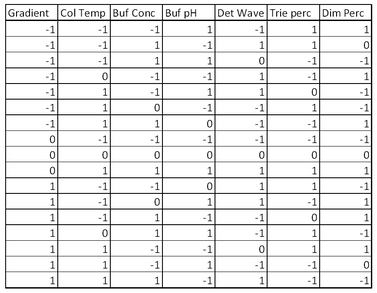
What do we learn from analyzing the DSD experimental data?
As in the previous blog post, we will illustrate the analysis by looking at the results for the peakHeight response in the HPLC application. Throughout, we divide the actual peakHeights by 1000 for ease of presentation. We proceeded to fit a model to the DSD experimental data that includes all main effects and pure quadratic effects. The analysis shows that the only significant quadratic effect is that for Gradient. In addition to the Gradient quadratic effect we decided to keep in the model, as linear main effects: Gradient, Column Temperature, Detection Wavelength and Triethylamine Percentage. In Figure 1, we show parameter estimates from fitting this reduced model to the peakHeight responses. All terms are statistically significant, the adjusted R2 is 87%, and the run-to-run variation has an estimated standard deviation of 2.585.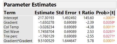

Finding a robust solution
In order to improve robustness, we need to identify nonlinear effects. Here the only nonlinear effect is for gradient. Figure 2 shows us that the quadratic response curve for gradient reaches a minimum quite close to the nominal value (0 in the coded units of Figure 2). Consequently, setting the nominal level of Gradient to that level is a good choice for robustness. The other factors can also be kept at their nominal settings. They have only minor quadratic effects, so moving them to other settings will have no effect on method robustness.
We can assess the level of variation, as in the previous post, by assigning normal distributions to the input factors. As in that post, we use the default option in JMP, which assigns to each input a normal distribution with standard deviation of 0.4 (in coded units). Figure 3 shows the results of this simulation. The standard deviation of peakHeight associated with variation in the factor levels is 2.697, very similar in magnitude to the SD for run-to-run variation from the experimental data. The estimate of the overall method SD is then 3.736 (the square root of 2.6972 + 2.5852).
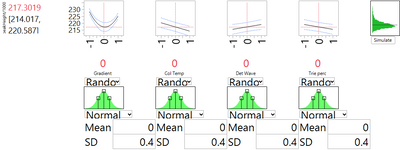
It is instructive to compare the results from analyzing the DSD to those from analyzing the fractional factorial in the previous blog post. Both experiments ended with the conclusion that gradient has a nonlinear effect on peakHeight, and that setting gradient close to its planned nominal level is a good choice for robustness of the analytic method. The fractional factorial was not able to identify gradient as the interesting factor; this happened only after substantial discussion by the experimental team. And even then, there was concern that the decision to attribute all the nonlinearity to the gradient might be completely off the mark. The DSD, on the other hand, with just a few more runs, was able to support a firm conclusion that gradient is the only factor that has a nonlinear effect. There was no need for debate and assumptions; the issue could be determined from the experimental data.
The DSD and the fractional factorial are both able to assess variance from factor uncertainty and both agree that the three factors with the most important contributions are gradient, column temperature and detection wavelength. The DSD identified a fourth factor, the percent of Triethylamine, as playing a significant role.
The DSD, by estimating all the pure quadratic effects, was also able to fully confirm that there would be no direct gain in method robustness by shifting any of the factors to different nominal values. Improvement might still be possible due to two-factor interactions; but as we pointed out, only a much larger experiment could detect those interactions.
Can we still improve method robustness?
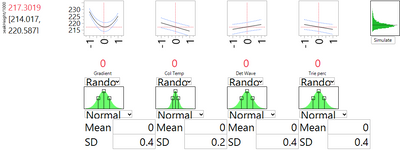
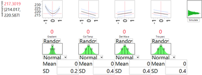
The DSD has shown us that changing nominal levels is not a solution. An alternative is to institute tighter control on the process parameters, thereby limiting their natural variation. Moreover, the DSD helps us prioritize the choice of which factors to control. Figures 1 and 3 show us that the strongest linear effect is due to the column temperature. They also show that the strong and nonlinear effect of gradient may be contributing some of the most extreme high values of peakHeight. Thus these two variables appear to be the primary candidates for enhanced control. Figures 4 and 5 use the simulator option with the profiler to see the effect of reducing the natural spread of each of these factors, in turn, by a factor of 2. With enhanced control of the column temperature, the SD related to factor uncertainty drops from 2.697 to 2.550. Reducing the variation of the gradient leads to a much more substantial improvement. The SD drops by about 40%, to 1.667.
Summary
Experiments on robustness are an important stage in the development of an analytic method. These experiments intentionally vary process factors that cannot be perfectly controlled about their nominal value. Experiments that are geared to fitting a linear regression model are useful for assessing robustness, but have limited value for improving robustness.
We have shown here how to exploit nonlinear effects to achieve more robust analytic methods. The Definitive Screening Design can be especially useful for such experiments. For a minimal experimental cost, it provides enough data to estimate curvature with respect to each input factor. When curvature is present, we have seen how to exploit it to improve robustness. When curvature has been exploited, we have seen how to use the experimental results to achieve further improvements via tighter control of one or more input factors.
Notes
[1] Jones, B. and Nachtsheim, C. J. (2011) “A Class of Three-Level Designs for Definitive Screening in the Presence of Second-Order Effects” Journal of Quality Technology, 43. 1-15.
[2] Borman, P., Nethercote, P., Chatfield, M., Thompson, D., Truman, K. (2007), Pharmaceutical Technology. http://pharmtech.findpharma.com/pharmtech/Peer-Reviewed+Research/The-Application-of-Quality-by-Desig...
[3] Romero R., Gasquez, D., Sanshez, M., Rodriguez, L. and Bagur, M. (2002), A geometric approach to robustness testing in analytical HPLC, LCGC North America, 20, pp. 72-80, www.chromatographyonline.com.
[4] Steinberg, D.M., Bursztyn, D. (1994). Dispersion effects in robust-design experiments with noise factors, Journal of Quality Technology, 26, 12-20.
You must be a registered user to add a comment. If you've already registered, sign in. Otherwise, register and sign in.
- © 2026 JMP Statistical Discovery LLC. All Rights Reserved.
- Terms of Use
- Privacy Statement
- Contact Us
