What is OFAT? What's wrong with it?
One factor at a time (OFAT) experimentation generally involves holding all but one factor constant, varying the remaining factor, and observing how this changes a response. Without close examination, OFAT seems to be an intuitive and "science-y" way to solve problems. Personally, before learning about the Design of Experiments (DOE) approach to experimentation, I never questioned OFAT as the default approach, even going as far as thinking that I couldn't vary more than one factor at a time any time I was trying to solve a problem. I remember once spending about three days with a process engineer trying to optimize a process using OFAT methods. I thought I was being methodical and scientific and solving the problem the right way while requiring the fewest resources. I was wrong. Upon examination, OFAT is neither a) good at finding the best process settings—-the sweet spot, nor b) an efficient use of resources.
Wait, OFAT doesn't find the sweet spot?
No, OFAT doesn't always find the best process settings. To see this, download and install the OFAT vs. DOE add-in, which generates a curved response for two process factors (called 'x' and 'y') and displays a graph of this response along with some buttons along the right side of the graph. The 'Scatterplot 3D' button generates an interactive way to visualize the shape of the response. The 'Toggle Visibility' button turns the view of the entire response surface on or off.
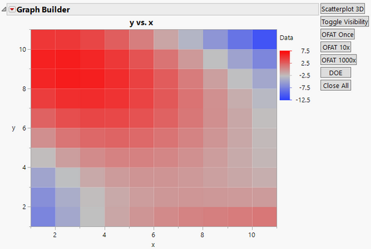
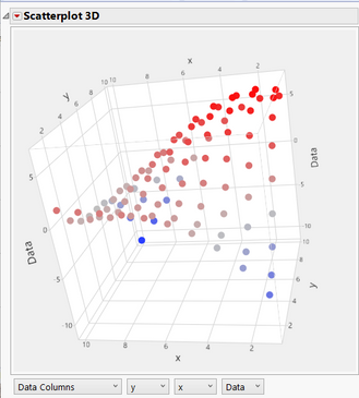
In this example, imagine trying to find the highest process output possible, which is in the x=2, y=8 square. The 'OFAT Once' button mimics one standard OFAT approach:
- Choose a spot at random.
- Holding all other factors constant ('y' in this case), vary the one remaining factor ('x') across the allowable space, seeking to find the maximum.
- From the maximum found, choose another factor to vary ('y' is the only one left in this experiment), hold all others constant, and seek the maximum.
- Repeat step 3 until all factors have been tested (not necessary in this case, as there were only2 factors total).
- Celebrate because you've found the sweet spot using science! But wait, are you sure?
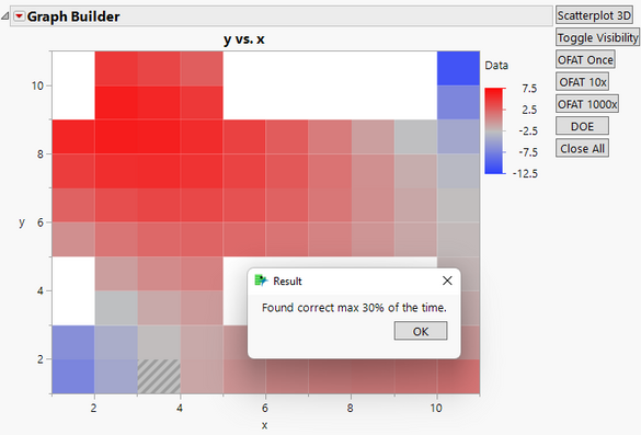
Try this out for yourself. Click the 'Toggle Visibility' button to clear the graph (to pretend you don't know what things look like already). Using the 'OFAT Once' button, watch how the experimental process unfolds. If you're lucky (about 20% of the time), you'll find the process maximum/sweet spot. The rest of the time, you'll end up not finding the maximum. Sometimes, you'll even end up in the lower right quadrant, thinking the maximum process output is about 1.5 units. Below is an example of a lucky OFAT experiment (left) and an unlucky one (right).
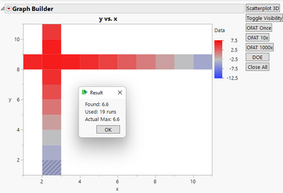
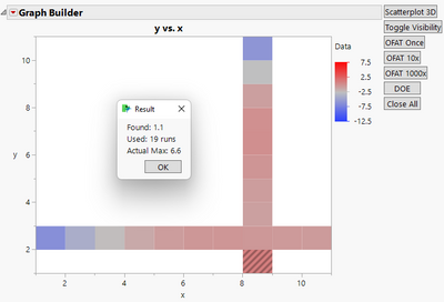
Use the 'OFAT 10x' button to simulate quickly running an OFAT experiment 10 times, and you'll see that the sweet spot is only found about 30% of the time (your number may vary because of random sampling).
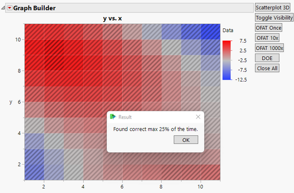
The 'OFAT 1000x' button quickly runs 1,000 experiments and outputs how often OFAT finds the sweet spot. Finding the sweet spot only around 25% of the time shows that OFAT experiments can't be relied on.
But surely OFAT is efficient. That fancy DOE approach will take more experimental runs, right?
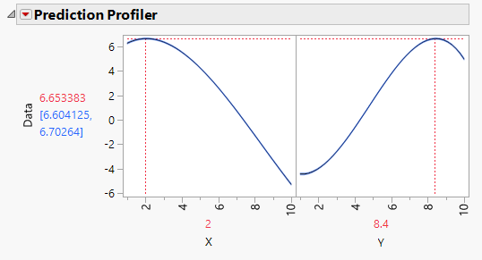
Wrong. DOE means fewer runs. Each OFAT experiment in the interactive script takes 19 runs (10 for the 'x' factor and 9 for the 'y' factor). The DOE button on the right side of the window opens a data table that includes the results of a DOE made in JMP's Custom Designer that includes all main effects, all 2-way interactions, all squared terms, and all cubed terms. JMP made this a 14 run DOE, and it not only finds the sweet spot, but also it generates a model that predicts the entire range of both factors, as shown in the profiler below (to interact with this profiler, run the 'Model' script in the DOE data table).
The results only get better as complexity increases. A process with 5 continuous factors using the same OFAT method would take 46 runs (10 for the 1st factor, 9 for each of the remaining factors) and might not even find the sweet spot. JMP's Custom Designer generates a design for the same five factors that takes only 12 runs (main effects only) or 27 runs (main effects, all 2-way interactions, all squared terms). These designs also include repeated runs, so an estimate of response variation can be calculated. Clearly, a DOE approach to experimentation is better than OFAT experimentation: DOE uses fewer experiments and finds the sweet spot more regularly.
That's a convincing argument in favor of DOE. Is there anything else?
Yes. In addition to finding solutions more often while requiring fewer resources, the DOE approach also generates a model that can be used to answer other questions about the factors being studied. With OFAT, if circumstances change, luck dictates whether new circumstances can be addressed without further experimentation. For example, what if the customer of the sample process above only needs a process output of about 1.5 units and ingredient 'y' becomes extremely expensive? An OFAT approach may not have an answer to this. A DOE approach has a model that can generate a new sweet spot of x=0 and y= 1.
What about your experience? Have you seen examples of these two types of experimental approaches in your work? Want to add something that I missed? Please comment below.
You must be a registered user to add a comment. If you've already registered, sign in. Otherwise, register and sign in.