- New to JMP? Let the Data Analysis Director guide you through selecting an analysis task, an analysis goal, and a data type. Available now in the JMP Marketplace!
- See how to install JMP Marketplace extensions to customize and enhance JMP.
JMP Blog
A blog for anyone curious about data visualization, design of experiments, statistics, predictive modeling, and more- JMP User Community
- :
- Blogs
- :
- JMP Blog
- :
- Optimizing Multiple Curves in the Functional Data Explorer
- Subscribe to RSS Feed
- Mark as New
- Mark as Read
- Bookmark
- Subscribe
- Printer Friendly Page
- Report Inappropriate Content
Introduction
The Functional Data Explorer (FDE) platform in JMP is a very nice tool to have when modeling curves or spectral data as outputs. But what if I have multiple curves as outputs? And what if each of those curves has a different priority to my business? Can JMP be used to model, compare, and optimize multiple curves at the same time? I've been asked these very questions a few times in the last month, and (of course) the answer is "yes." Read on to find out how.
Background
I'll use a slightly modified Mill DOE.jmp from the Sample Data to make this example. The file is attached to this blog entry. The data represents a designed experiment to optimize a roller mill process, with the goal being to have the size curve shrink rapidly. I've added a column which tracks power usage during each experimental run. The goal for this column is to minimize power usage during the process. I've also added a target batch to the data as Batch 0 and I've removed some of the other columns in the data table.
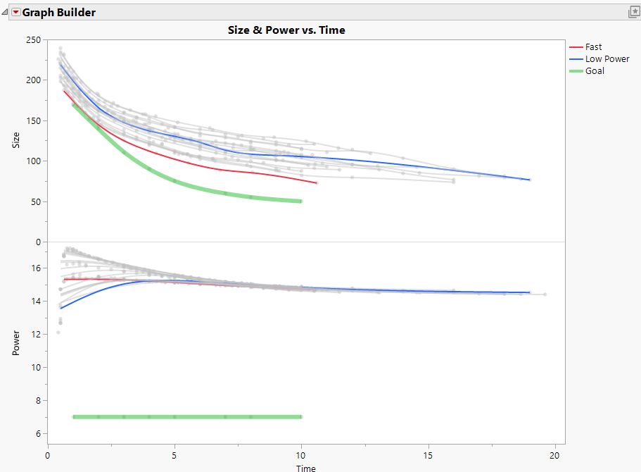
This is now a good data set to illustrate how to optimize competing curves: I'd expect that using more power will cause the process to reduce the particle size faster, and I'd hope that there is a happy spot in the design space where power usage can be low and where the milling process can be quick. In the graph below, I can see that the fastest DOE run (red line) is near the middle on power usage, and the lowest power usage (blue line) is largely in the middle for the milling process time. The green lines represent target curves for each output.
Functional Data Explorer
I'm assuming that readers will already know how to use the FDE platform. See this excellent overview by @Peter_Hersh if you need a refresher.
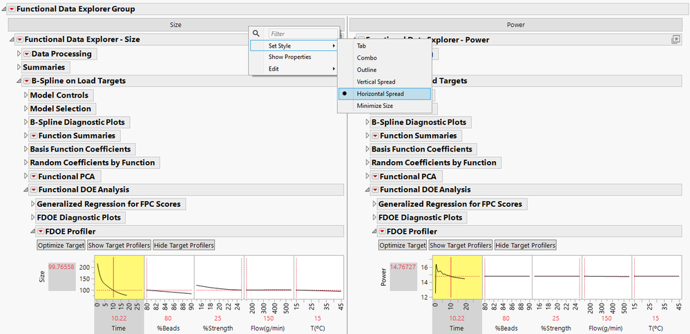
Focusing on multiple outputs at once is easy. Once I loaded the targets for each output, I fit B Spline models to each, then I right-clicked on the Tab Box at the top and selected Set Style > Horizontal Spread so I could see both profilers side by side. Once the profilers are linked (click on the profiler red triangle and select Factor Settings > Link Profilers), I can see tradeoffs as I optimize one output. It makes sense that the fastest size happens at the high beads, high bead strength, low coolant, high temperature corner. Likewise, the lowest power usage comes from a different corner where temperature and flow are low.
Process for getting both curves
What I can't do yet, though, is tell JMP which curve is more important and then use JMP's tools to automatically find the sweet spot where the process is both quick and inexpensive. There are at least two methods for doing this:
Method 1: Saved Column Formulas
This method won't work for every situation, but it's very fast and simple. If my target curves are always either above or below all the other curves, i.e., if I'm trying to maximize or minimize a curve, then I can save the formulas for each curve and use the Prediction Profiler to see and optimize both processes at once.
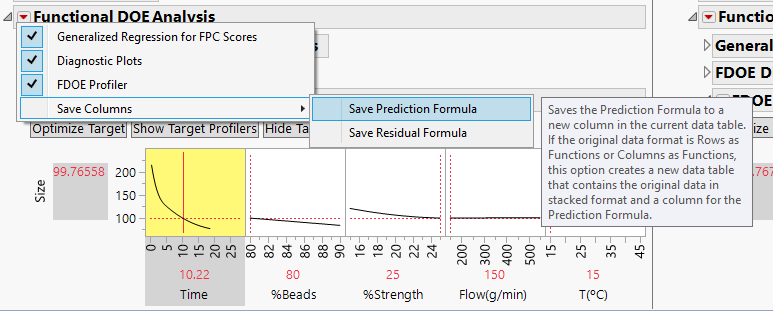
- For each of the curves, select the red triangle in Functional DOE Analysis. Select Save Columns > Save Prediction Formula.
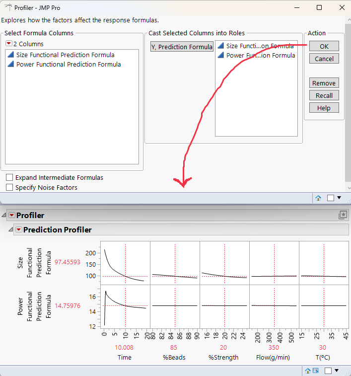
- Select Graph > Profiler, then select the prediction formulas, and click OK to continue.
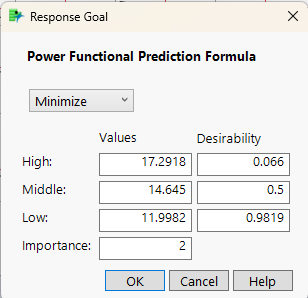
- In the Prediction Profiler red triangle, select Optimization and Desirability, turn on Desirability Functions, then return to that menu and select Set Desirabilities. In the windows that pop up, select Minimize, then assign an importance of 1 to Size. Next, select Minimize again, but this time set the importance for Power to 2. This would mean Power usage is twice as important as the size profile.
- Alt-click on any of the curves in the Time section of the Profiler, then select Lock Factor Setting and click OK. (Locking it keeps the Profiler from thinking it can move to different places on the curve as part of the optimization process.) Next, in the Optimization and Desirability menu, select Maximize Desirability. Changing the importance levels of each curve, then selecting Maximize Desirability again will change where the sweet spot is.
Method 2: JMP does calculus
The first method only works if I'm trying to minimize or maximize a curve. It fails if I need to match a specific curve that isn't a maximum or minimum. When one or more of the curves needs to fit a shape that isn't a maximum or minimum, outputting an intermediate table and then fitting a model to that table makes it possible to optimize multiple functional responses. To accomplish this, I'll go back to my original FDE output:
- Alt-click in the white space of the Profiler for Time on the Size output; ensure Lock Factor Setting is selected, then click OK. Repeat this on the Power output. If the profilers are already linked, the second output will automatically be locked. Locking this factor makes the output of the next step much smaller.
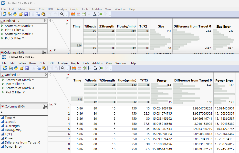
- Click the red triangle near the FDOE Profiler for Size, then select Output Grid Table.
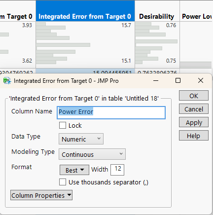
- In the Table that pops up, rename the column “Integrated Error from Target 0” to “Size Error.”
- Repeat Steps 2 and 3 for Power, renaming the “Integrated Error” column to “Power Error.”
- To simplify things, you can delete all the columns in both grid tables, after the “Error” columns you previously renamed.
- Use the Tables > Update tool to combine the two tables. You'll need to match all the first five columns, but this doesn't mean lots of clicks: just select all options between Time and T(°C) in both column groups, then select Match.
Now all I need to do is fit a model to minimize the error of each of my responses. A neural network is a good choice here.
I can set Desirabilities similar to the previous method. In this case, however, I want to minimize the error from the target curve for each of my responses. What's nice about this method is that it works for any target curve. If I set the relative importance the same as before, with Power being twice as important as Speed, the sweet spot I get is to have every input at maximum except for Flow, which I'd want to set at the minimum. Even better, since I still have my original FDE platform open with profilers side by side, I can see what my outputs will look like automatically, since all three profilers are linked.
Conclusion
There are likely all sorts of reasons why a person might want to optimize multiple curves simultaneously. For example:
- For automobiles, fuel efficiency and engine power output curves.
- For drug development, dissolution curves and NMR spectroscopy.
- For financial gurus, pitting various risk-return curves against each other.
With the two methods outlined above, each of these situations can be addressed, and since all the functional data is being used, the answers come much faster and with much greater accuracy.
You must be a registered user to add a comment. If you've already registered, sign in. Otherwise, register and sign in.
- © 2026 JMP Statistical Discovery LLC. All Rights Reserved.
- Terms of Use
- Privacy Statement
- Contact Us

