- New to JMP? Let the Data Analysis Director guide you through selecting an analysis task, an analysis goal, and a data type. Available now in the JMP Marketplace!
- See how to install JMP Marketplace extensions to customize and enhance JMP.
JMP Blog
A blog for anyone curious about data visualization, design of experiments, statistics, predictive modeling, and more- JMP User Community
- :
- Blogs
- :
- JMP Blog
- :
- MANOVA test-statistics
- Subscribe to RSS Feed
- Mark as New
- Mark as Read
- Bookmark
- Subscribe
- Printer Friendly Page
- Report Inappropriate Content
Last time on multivariate analysis…
In my Sassy Statistician blog, we learned that the MANOVA is just like the ANOVA…with a few tweaks. Just like the ANOVA, the MANOVA partitions variance into parts, but now the variance is in the form of a matrix instead of a one-dimensional number.
We took our Variance matrix (called the sums of squares and cross products) and partitioned it into two matrices: The “between” matrix, which represents the variance of our group mean vectors around the overall mean vector, and the “within” matrix which represents the variance of the data vectors around their group mean vectors. We’ll call these matrices H and E for Hypothesis ("between") and Error ("within").
I left you with a cliffhanger about how to conduct a hypothesis test with these matrices, and now I am here to deliver.
Let’s talk about hypothesis testing in a MANOVA.
The ANOVA uses the partitioned 1d (one-dimensional, not OneDirection) variance to create an F-ratio comparing variance between groups to variance within groups. The MANOVA does the same thing, but we start with a matrix of variance and covariances.
We want to compress a matrix into one number so that we can compare it as easily as we compare 1d variances in an ANOVA. But there’s many ways to skin a cat…I mean…compress a matrix, and all of them are valid. Perhaps for this reason, there are many test-statistics for a MANOVA. We’ll talk about four – that’s right, four – of the most common.
WILK’S LAMBDA
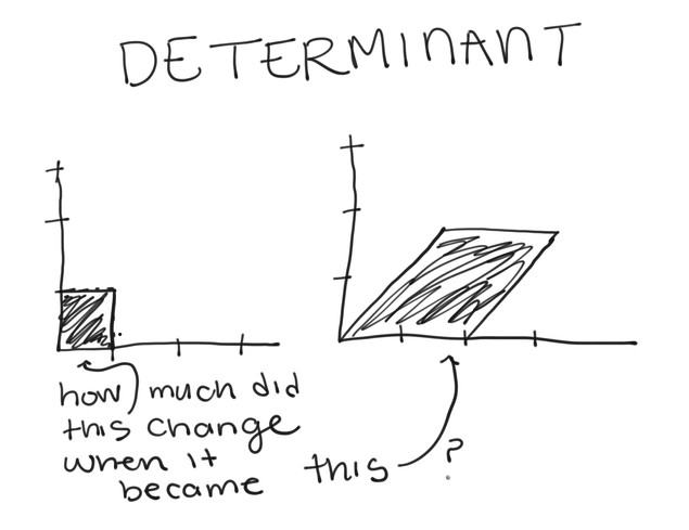
We begin with Wilk’s Lambda. Wilk’s Lambda uses determinants to compress matrices in to one-dimensional numbers. First, a quick refresher on determinants.
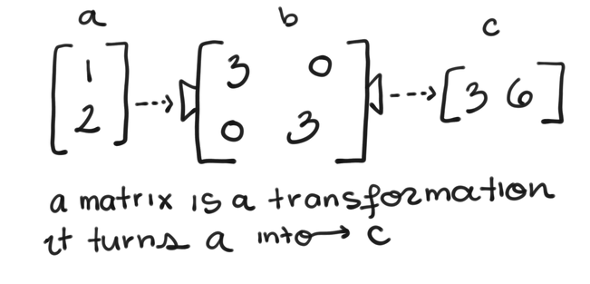
A matrix is really a transformation because when you multiply something by a matrix, it moves and stretches that thing. For example, the matrix ![]() takes the vector
takes the vector ![]() and changes it to the vector
and changes it to the vector ![]()
The amount of “stretching”– or conversely, “squishing”– a matrix does is represented by its determinant. Matrices that stretch things have large determinants, and matrices that squish things have small determinants.
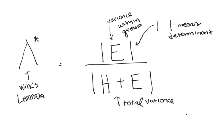
Wilk’s Lambda is the determinant of our E matrix, divided by the determinant of H+E. This gives us an idea of how “big” the within group variance matrix is compared to the total variance matrix (remember in our example, H+E = Total Variance) because the amount a matrix stretches things is a way of measuring how big a matrix is.
If there was an effect in our data, we’d expect E to be a smaller part of the total variance (H+E) than H. Since the determinant tells us how much a matrix stretches an object, and Wilk’s Lambda ends up being a ratio of how much the E matrix stretches things, compared to how much the matrix (H+E) stretches things. If E stretches things only a little compared to (H+E), we will get smaller Wilk’s Lambda. Unlike with the F-statistic in an ANOVA, we tend to reject the null then Wilk’s Lambda is small. The rejection criteria for Wilk’s Lambda is a bit more than I want to get into here, so I’ll leave that particular calculation up to your statistical software.
HOTELLING-LAWLEY and PILLAI TRACES
The next two test-statistics use something called the trace of a matrix, so a quick recap before we start.
The trace of a matrix is the sum of the diagonal elements of a matrix. It doesn’t have a clear geometric interpretation like the determinant, but the two are related. What I didn’t mention before, is that the determinant is equal to the product of the eigenvalues of a matrix. For more on eigenvalues, I recommend 3Blue1Brown’s video on the subject.

Eigenvalues each have a matching eigenvector. When we think about a matrix as a transformation that takes in an object and stretches it; the eigenvectors represent the direction (or axis) that the object is stretched, and its eigenvalue friend tells you how far it’s stretched. The determinant is the product of all the eigenvalues, the trace is the sum of them. While they don’t give us exactly the same information, the source is the same.
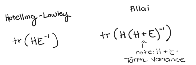
All right enough about traces. Let’s look at the two test-statistics that use them: the Hotelling-Lawley Trace, and the Pillai Trace. Oops, I guess we’re still talking about traces.
The Hotelling-Lawley version takes the trace of the matrix
If H is large compared to E, then the Hotelling-Lawley trace will be BIG, unlike Wilk’s Lambda, so we reject when the trace is significantly large.
Similarly, the Pillai version takes the trace of the matrix
Remember H+E is the total amount of variance, so again, if H is large compared to the total variance matrix (H+E), then the Pillai trace will be large.
ROY’S MAXIMUM ROOT
The fourth and final test-statistic is also a derivative (not in the calculus sense) of the eigenvalues of our H and E matrices, but this one is a little simpler. Roy’s Maximum Root is the maximum eigenvalue of
An eigenvalue is a “root” of the characteristic polynomial of a matrix, more on that here.
Just like with the Hotelling-Lawley Trace,
will be large if H is large compared to E. But since we use only the largest eigenvalue instead of some combination of all of them, Roy’s Maximum Root often overestimates an effect. So, if you ever run into a case where none of the other test-statistics are significant but Roy’s Root is, the significance of Roy’s root is most likely a false positive and should be ignored.
That’s it, you’ve made it through all of test-statistics and matrices, and we’ve nearly reached the end of this article. You may notice that I haven’t covered p-values here, but your statistical software will give you a p-value associated with each of these test statistics based on each of their distributions.
In JMP, running a MANOVA is just as easy as running any linear model. You put all of your outcome variables into the Y box, your predictors into Model Effects, and switch the Personality to MANOVA.
Once you click Run, JMP will pop open a window for your MANOVA, but you've still got to choose your Response Specification. For a basic MANOVA, JMP reccomends choosing the Identity option, but see here for other contrast matrices you can use.
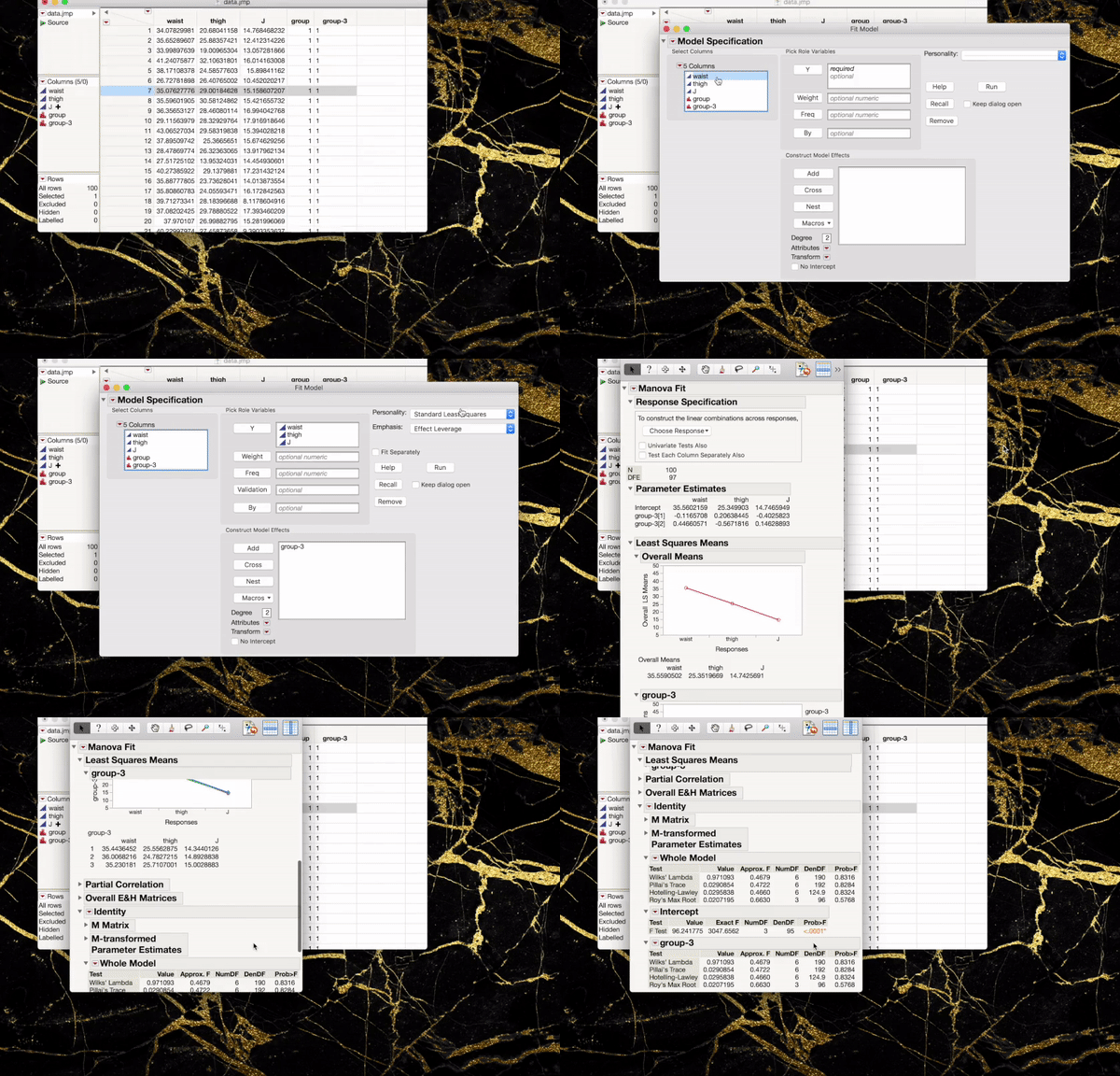
With the contrast matrix chosen, you'll now see your beautiful MANOVA test statistics pop up in the window. Just like with the ANOVA, you'll see a test for the Whole model, the intercept, and one for each effect you've put in your model (here we only have one, group).
Notice how the intercept effect only gives an F test and not our newly learned test statistics? JMP automatically does this for any and all effects, which have one degree of freedom. With one degree of freedom, the test statistics are equivalent, so JMP consolidates for you and simply reports just the F-test.
Just like the ANOVA, the MANOVA is an omnibus test, meaning that a significant test means there’s some difference somewhere, but it won’t tell us where it is. When you get a significant ANOVA, you’ll have to test each pair of groups to see where the difference in our outcome variable is. In a significant MANOVA with more than two groups, and more than two outcome variables, you will not only be unsure of which groups are different, but which outcome variables are responsible for that difference. The MANOVA just tells you there is a difference, not where it is. For that, we’ll need some follow up tests. But more on that later.
- © 2026 JMP Statistical Discovery LLC. All Rights Reserved.
- Terms of Use
- Privacy Statement
- Contact Us








You must be a registered user to add a comment. If you've already registered, sign in. Otherwise, register and sign in.