- New to JMP? Let the Data Analysis Director guide you through selecting an analysis task, an analysis goal, and a data type. Available now in the JMP Marketplace!
- See how to install JMP Marketplace extensions to customize and enhance JMP.
JMP Blog
A blog for anyone curious about data visualization, design of experiments, statistics, predictive modeling, and more- JMP User Community
- :
- Blogs
- :
- JMP Blog
- :
- Lessons learned in modeling Covid-19 (Pt 2)
- Subscribe to RSS Feed
- Mark as New
- Mark as Read
- Bookmark
- Subscribe
- Printer Friendly Page
- Report Inappropriate Content
Previously, on "Lessons Learned"...
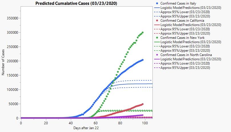
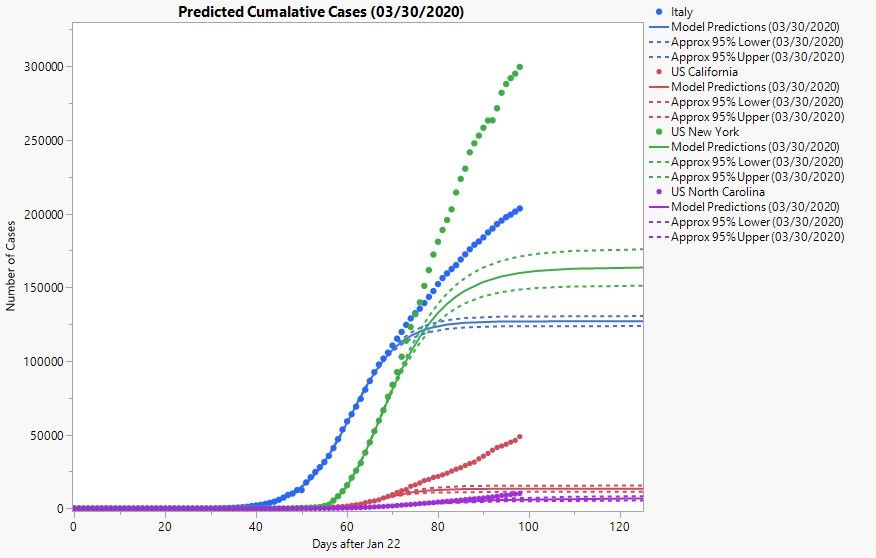
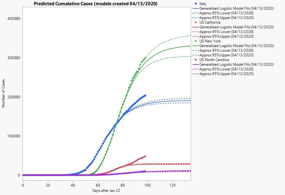
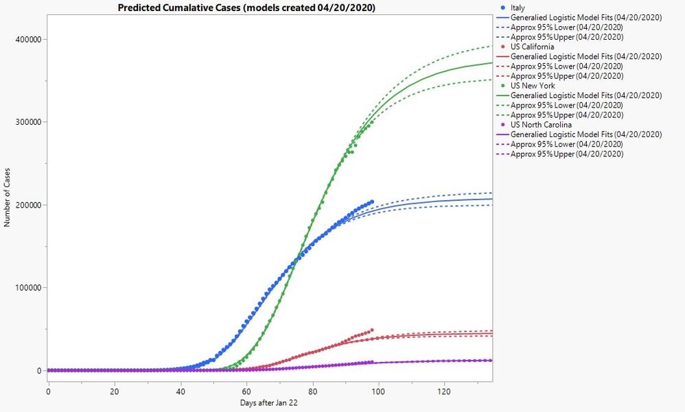
Whelp, I’m still at home and still trying my hand at this whole statistical modeling thing. When last you left me (thanks for coming back!), I seemed strangely optimistic and resilient to the fact that my predictive models had been performing so poorly. Since then, my initial models have continued to tank. In fact, here is a plot of all four along with the current counts up to the writing of this blog post (April 30, 2020).
Yeeaaah, it’s not pretty. Maybe as abstract art, but not as sound predictive models that’s for sure. But, much like heroes of page and screen, adversity has caused me to adapt, and even learn new things!
If at First You Don’t Succeed…
The first thing I realized is that my model had additional limitations beyond those discussed in the first post. Specifically, a logistic model assumes that the rate of change is symmetric around the inflection point. How fast the cases rise from 0 is the same as the rate at which it approaches the asymptote. This might have been too restrictive for some of the data, so I decided to try fitting other types of sigmoid curves. At this point, I found myself tempted to start “dart modeling.”
Dart modeling? What’s that? Well, it’s my term for when someone performs model fitting by picking random models and “throwing” them at the data to see which one sticks best. Much like throwing darts at a dartboard (though my “dart modeling” game is probably better than my actual “darts” game). “Well, what’s wrong with that?” you might ask. Hmm…I guess there’s nothing really “wrong” per se. I don’t frequent many bars, especially those with dartboards, so I guess it’s not really an issue that I’m not that good at – oh, you meant “dart modeling”! My bad.
Yes, on the surface, it sounds like I’m dissing the entire point of statistical modeling. But hear me out. I agree that fitting different models is good practice. It helps prevent yourself from being biased to a particular model, much like what was happening with my logistic models. At the same time, there’s a strong tendency to just slap on many different types of models and, when one seems to perform well, make the fit, check the metrics, get the predictions, publish the report, pour yourself your favorite beverage, get comfy in your favorite chair, lean back, and enjoy a job well done. But that’s missing one of the most important (if not the most important) aspects of statistical modeling! Let me summarize it this way: A good model fits and predicts well; a great model improves and engages your understanding.
Teach a Man to Fish…
Using a particular model or distribution solely because its fits and predicts well enough without truly understanding where that model comes from is like hanging an original Rembrandt or Salvador Dali on your bathroom wall solely because it helps cover up a blank wall; it does the job, yes, but that’s completely missing the point. Let’s take the ever-popular Normal or Gaussian distribution, for example. It pops up all over the place in statistical modeling, but I would wager that very few people know where it originated. Knowing this history provides valuable context to when and where it is appropriate to use such a distribution. However, for most people, it’s a gold standard their data must adhere to (or can be forced to adhere to), or else they’re sunk. This is very saddening; if there is a discrepancy between the data and the model, it should be seen as an opportunity for discovery and not as a failure of the data to meet your standards. If it’s a contest between data and model, the data should win more often than not.
In the case of my modeling of COVID-19 confirmed cases, my realization of the limitations of using a logistic model led me to consider other types of sigmoid models. I next considered a Gompertz model because it seemed like the next logical choice. …OK, OK, you got me. It was actually just another fancy sounding option in JMP’s sigmoid model collection, so I thought I’d give it a try. However, some quick research did show that it had been used in disease modeling, so worth a shot right? I can just see Dr. Fauci hanging his head in shame.
Actually, that quick research led to something more. Much more. First, I found that the Gompertz and logistic models were both part of a family of models called generalized logistic models or Richards curves. The family of curves have the following common form:
I(t)=A/{1+e^[-b(t-t0)]}^v
where A is the asymptote, b is the rate of increase, t0 is the inflection point, and v is a fourth parameter that controls on which side of the inflection point the rate of increase is fastest. If v<1, then the rate of increase is fastest before the inflection point. When v=1, you get the logistic model I had been using up to this point. Practically speaking, this would mean that the number of daily cases will take longer to drop after the peak (inflection point) than it did for them to increase prior to the peak. I actually fit this model to the data using the Nonlinear platform in JMP and got pretty good results. But even in this, I think I was still missing the point of the generalized model. With occasional exceptions, these types of models are typically used to be more flexible in modeling and ultimately help narrow down to a more specialized model. In this case, I was finding that the value of v I would be getting was very, very small. To the point of practically being no different from zero. As it turns out, as v->0 in the limit, the generalized logistic function becomes a Gompertz function. So my choice wasn’t as haphazard as I thought!
The next thing I learned was perhaps even more enlightening. As I was looking over these models, I wondered if there was any connection to epidemiological models. The short answer is yes, there is. But the long answer is more fascinating, so we’ll walk through it.
The simple logistic model I was using is actually the solution to the pair of differential equations that arise under an SIS model for epidemics. Here, S stands for Susceptible and I stands for Infected. This model is a simplified case of an SIR model (where R stands for Removed or Recovered) where, instead of moving from Susceptible to Infected to Recovered, you simply switch from Susceptible to Infected back to Susceptible. In other words, this model is appropriate for situations in which an immunity to the disease never fully develops, such as with the common cold. Now, how appropriate this model is for something like Covid-19 is something I will defer to the epidemiologists. But at least there is some connection to a well-known epidemiological model, even if it is a very simple one.
To better understand this connection, let’s take a look at that solution I mentioned, which looks like this:
I'(t) = C I(t){1-[I(t)/A]},
where C is a proportionality constant.
This solution means that the rate of infection, I’(t) is proportional to the current level of infection weighted by the distance of that level to some upper bound A (typically the population of the location of interest). That is, as the counts of infection increases, it does so more quickly initially because that weight is small (I(t) is far from A) but then slows down after a while as I(t) gets closer to A. This interplay between the counts and its distance from A is what leads to that S-shaped sigmoidal behavior.
What about the Gompertz model? Unfortunately, I’ve not yet been able to find the connection between it and one of the many epidemiology compartmental models. Maybe there’s someone out there who does? Please comment if you do! If not, then that just means we have an opportunity for discovery right? At the very least, I know of some people who have fit the Gompertz model in published research and even fellow JMPers/armchair analysts have seen its potential (see @matteo_patelmo's excellent comment on my first post)! Which leads me to another discussion point…
Zoom…It’s Not Just an Online Chat Tool
As I read through articles, Twitter posts, and calls for research on Covid-19, I often find myself feeling inadequate. There are a lot of epidemiologists out there doing very hard work to try and understand this virus. The best I can do is say that the observed trend in Covid-19 cases follows some type of model with some connection to disease modeling. Does this mean my approach is less informative?
As I pondered this, I was reminded of how we teach physics. Seems a bit of a stretch, I know, and some of you may have bad memories of the subject, but hear me out. When you’re first taught physics, you start with Newton’s laws of motions, studying the movement of things like swinging pendulums, springs, cannonballs flying through the air, and the orbital motions of planets. All pretty fascinating stuff! But, for those who continued their studies into college and maybe even beyond, you started to “zoom in” and began studying the movements and interactions of atomic and even subatomic particles. It all seems so advanced and complicated. Yet, in theory, you could use those same complex interactions to describe how a ball thrown the air makes the arc that it does, ultimately coming up with the same quadratic equation you derived in that high school physics class. You could argue the same thing is happening with the disease modeling going on right now. Some of us, including myself, are taking a “zoomed out” approach, modeling the number of confirmed and daily cases with relatively simple models that describe the basic trends. Others, like the epidemiologists, are taking a “zoomed in” approach, trying to model the same phenomena but using their subject matter expertise regarding how diseases behave and spread.
All this is to say that, whether you are “zoomed out” or “zoomed in,” we both should converge on the same goal. Whether from 30,000 feet up or standing among the trees, a forest is still a forest. That’s why I was so excited to see the connection between the logistic model and the SIS compartmental model. It validated my approach by showing it was a different way of describing the same thing. It’s why I also have hope about the Gompertz model. Perhaps somewhere, out there, there’s a “zoomed in” companion just waiting to be found (or explained to me).
The Road Goes Ever On and On…
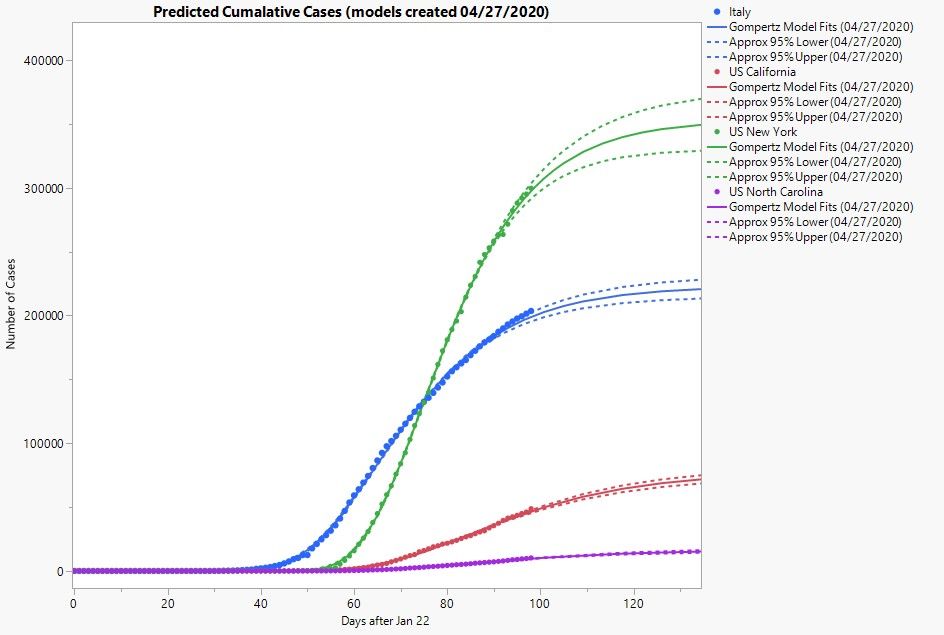
Well, so long as we are under stay-at-home orders, I’ll be continuing my statistical modeling adventures. If you’re wondering how well my new models have been performing, here’s a quick look as of April 29, 2020.
Looks like I’m doing much better! Though having an additional month’s worth of data certainly helps. For the sake of openness, here’s all of the models I’ve been using over the past month shown with all of the data up to April 29, 2020.
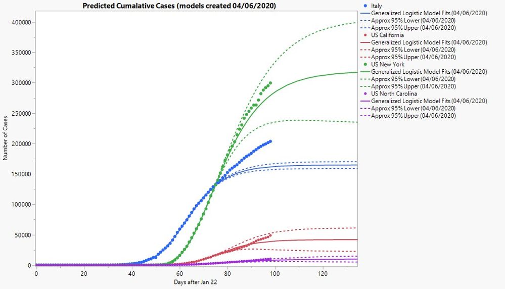
You can clearly see a lot of back and forth in how well my models captured future observations. At one point, I did use a mixture of Gompertz and logistic models before ultimately switching to the generalized logistic models, fitting them with the Nonlinear platform in JMP. It was only recently that I noted the parameter estimates were all leaning toward a Gompertz model, which is I why I ultimately switched back to that particular model.
I'm also attaching some of the data I've been using here in this data table should you wish to try your own hand at modeling (and learning). It also contains my model fits over time as well as some other helpful table scripts. Note that it only contains data up until the end of April. Should you wish to add on to it, feel free to visit the John Hopkins University CSSE site, which has been my primary source.
I will add a quick note of caution if you are considering publicly posting your predictive models. As I talked about in this blog series, predictive modeling is a tricky business. There is already a great deal of questionable results and misinformation out there. So please, consider carefully before you post.
I hope you’ve enjoyed following along on my statistical modeling journey and maybe learned something new! So until our next meeting, stay home, stay safe, and stay curious!!
You must be a registered user to add a comment. If you've already registered, sign in. Otherwise, register and sign in.
- © 2026 JMP Statistical Discovery LLC. All Rights Reserved.
- Terms of Use
- Privacy Statement
- Contact Us

