- New to JMP? Let the Data Analysis Director guide you through selecting an analysis task, an analysis goal, and a data type. Available now in the JMP Marketplace!
- See how to install JMP Marketplace extensions to customize and enhance JMP.
JMP Blog
A blog for anyone curious about data visualization, design of experiments, statistics, predictive modeling, and more- JMP User Community
- :
- Blogs
- :
- JMP Blog
- :
- Is that model any good?
- Subscribe to RSS Feed
- Mark as New
- Mark as Read
- Bookmark
- Subscribe
- Printer Friendly Page
- Report Inappropriate Content
In a recent edition of Technically Speaking, we saw how to incorporate variables derived from text mining into a predictive model in order to improve model performance. (If you haven’t watched the presentation, you may want to before reading on.) The case study focused more on the text mining than the predictive modeling, so let’s now look at two main modeling steps that weren’t discussed: namely, validating the model and scoring new observations.
Model validation
In predictive modeling, it’s crucial to test the model’s accuracy before using it to generate predictions. We want to ensure our model isn’t “overfit”, accurately capturing the data it was trained on but generating inaccurate predictions for data it hasn’t seen before. A great meme capturing the concept of overfitting has been circulating the Internet for a while now.
One way to check for overfitting is to set aside or “hold out” a subset of our data, train the model on the remaining data, and then test the model on the holdout set. We measure the model’s prediction performance on both the training and holdout data, and if we see a large drop off in accuracy from training to test sets, we have evidence our model is overfit.
We actually used this holdout validation procedure when building the Bootstrap Forest model in the case study, though we glossed over it. A table of model fit measures from the validation procedure is below. JMP provides a number of measures along which to compare training and test set performance (if you’re curious, read about them here); we saw Entropy RSquare and Misclassification Rate for the test group in the presentation. None of the measures shows a steep drop in performance from training to test (though there are some slight drops on a couple measures, which is not unusual), so we conclude our model isn’t overfit.
You may notice something: there’s a “Validation” column in this table, too. What’s that about? In actuality, we split our data into three subsets here: training, validation, and test. In our Bootstrap Forest model, the training set is used to find the best splits in each decision tree, while the validation set is used to decide when to stop making new splits in each tree as well as when to stop making new trees. That is, the model fitting algorithm keeps going so long as each new split or tree results in improved performance on the validation set. Once performance on the validation set levels off, the algorithm stops. (Remember that Entropy RSquare statistic? That’s the validation statistic used in this process.) Once the algorithm stops, the resulting model’s accuracy is assessed using the test set. In JMP Pro, all this happens automatically by specifying a Validation Column in the model specification window, as you saw in the presentation.
Not all models require three-part validation like this. It’s only necessary for models that use an iterative fitting procedure and a separate data subset (the validation set) to decide when to stop fitting. For models that don’t involve an iterative fitting procedure – logistic regression, for example, which we could have used here – only training and test sets are needed.
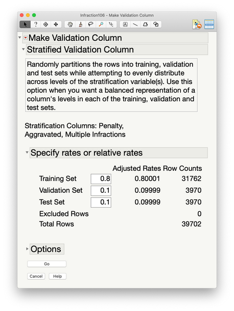
JMP Pro has an easy way to divide up our data for model validation. We used the Make Validation Column utility, which performs random or pseudorandom sampling (without replacement) on our data to create each subset, with the subsets recorded in a Validation Column back in our data table.
Here we used stratified random sampling to create our subsets, which is explained in the paragraph at the top of the second screenshot. There was strong imbalance in a few of our categorical variables, and we wanted to avoid a situation where, for example, few or none of the aggravated violations ended up in the test set. This would be problematic, because we need to see how the model performs on aggravated violations to get a valid measure of the model’s accuracy.
You can see in the interactive Distribution report below that we have a matched representation of each stratification column across our three data subsets. With nearly 40k rows of data, there’s a decent chance we would’ve been fine without using stratification, but it wasn’t a bad idea to play it safe. Stratification is one of several different pseudorandom sampling procedures that the Make Validation Column utility can implement (see here for more).
The Make Validation Column utility dropped a column named “Validation” back into our data table (which is available for download on the Technically Speaking presentation page), and we then fed that into the Bootstrap Forest platform to trigger the validation process. We didn’t find evidence of overfitting, so assuming that we’re comfortable with the model’s overall accuracy, we’re ready to use it to generate predictions for (“score”) new observations.
Scoring new observations
Imagine we have a group of building code violations just issued, and we want to assign a financial penalty probability to each one, which we’ll use to weight each levied penalty amount in our financial projections. For example, a levied penalty of $1,000 for a violation with a penalty probability of 0.7 would have a predicted payment of $700. Of course, the respondent ultimately will pay either $1,000 or $0, but on average across many violations, the sum of our projections should approximate our final revenue (we hope). We get the penalty probabilities out of our Bootstrap Forest model, but that model took as inputs the scores from the Topic Analysis. So we need to run our new violations through both models. This is not an uncommon practice, using the output of one model as input to another.
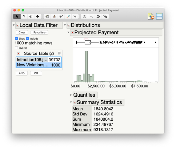
JMP can output models as column formulas back to the original data table (under the red triangle options in the modeling platforms), and they’ll run on any new data we add to the table. To score new observations, we simply add the new violations to our table, and the topic scores and penalty probabilities are calculated automatically by the column formulas. We then create a new column formula that multiplies the penalty probabilities by the levied penalty amounts, and we get our projected payments. Below we have projections for 1,000 new violations. We predict these will net us about $1.84m in revenue, though approximately one third of that total is accounted for by only the largest 100 projected payments in that positive tail. Our projection’s accuracy will hinge in large part on what happens with those violations.
(An aside: We’ve described the point-and-click way to score observations, but scoring could be automated easily through scripting in JSL (JMP Scripting Language). The model could also be deployed outside of JMP in a language like Python or JavaScript, with JMP Pro’s ability to write scoring code in other languages.)

A parting thought
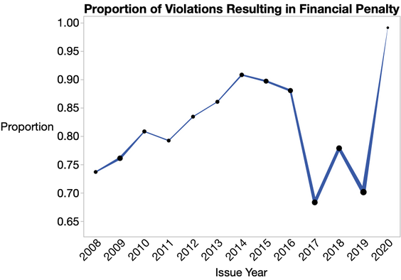
While we’ve arrived at our goal – a model that assigns financial penalty probabilities to new violations – a project like this is never truly done. Over time, new types or trends in violations may arise, new policies may alter the relationship between violation characteristics and penalty payments, or penalty payment probabilities could simply change over time due to unmeasured factors like enforcement capacity or leniency. The trends across time in the graph below might suggest the latter. (Line width represents total violations per year, which makes clear that we don’t have enough data in 2020 yet to trust the sudden rise this year.)
For many possible reasons, our model may become less accurate as time passes. We should refit our Topic Analysis and Bootstrap Forest models periodically, incorporating the latest data (and perhaps discarding older data) to ensure that our predictions remain accurate.
You must be a registered user to add a comment. If you've already registered, sign in. Otherwise, register and sign in.
- © 2026 JMP Statistical Discovery LLC. All Rights Reserved.
- Terms of Use
- Privacy Statement
- Contact Us


