The best way to make an impact when sharing your statistical discoveries is with compelling graphical output – an area where the data visualization paradigm of JMP is ideal.
 This four-part blog series will look at some of the options you have for exporting your visualizations created in JMP to graphic files that are ideally suited to your needs.
This first article will look at the graphical output options that are available. The second will focus on preparing graphics created in JMP for publication. The third will be a step-by-step video tutorial that explains the output process. Finally, in the fourth installment of this series, I’ll highlight some exciting options that will be available in the upcoming release of JMP 10 regarding graphical output. You won’t want to miss that!
JMP has many options for taking the visualizations generated in various platforms and saving them for use in other media – whether that is a report, Web page, print document or presentation.
Because the goals for these different output destinations are varied, it is important to understand the options for graphical output in JMP and to know which file types are most appropriate to your output destination.
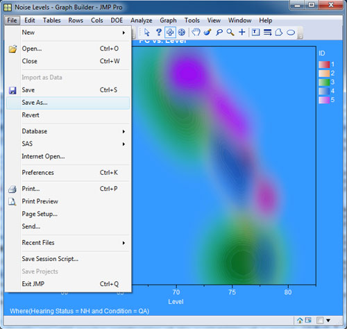
JMP makes it easy to save a figure using the selection tool. Just select the part of the graphic that you desire to output from JMP and then click on File -> Save As. This is shown in the figure below: The elements highlighted in blue will be output to a file when you save them. You can save the selection within a report that you choose to highlight in a variety of graphic output formats.

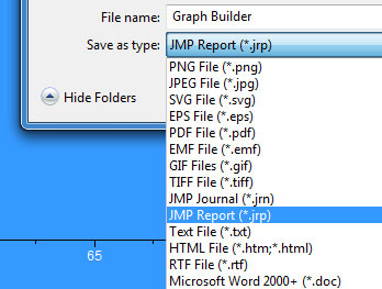
These include:
Additionally, you can save the selection as a JMP Journal, JMP Report, text file, HTML File, RTF File or a Microsoft Word 2000 + File. Since we are going to assume for the sake of this article that you are interested in using the output in something else (whether that be a report, presentation or print document), we will concern ourselves with the options for standard graphical output listed in the above list. In the figure below, you will see the options available when you select Save as type in JMP.

There are generally two file formats that I output my graphs from JMP in. The first is a .tiff file, and the second is a .eps file. I use the .eps files for any graphics that will need to be printed at a high resolution. I will explain why I choose this format over the other options in the second installment of this blog series.
The details of each file format is outside the scope of this overview article, but there are basically two types of graphical output formats: scalable, vector formats and fixed-scale, bitmap formats. Files saved as .png, .gif, .jpg and .tiff are bitmap formats that are either lossy (.gif or .jpg) or lossless (.png and .tiff). Lossy means that the file format is compressed to minimize the data storage requirement of an individual file at the expense of discarding some of it. While a .jpg image saved from JMP might be 29 KB, a .tiff image of the same dimensions might be 336 KB, or 11 times larger in size.
This size differences becomes an issue when you are outputting files for display in a presentation or online. You can run into memory issues quickly if you have users trying to look at a Web page that has multiple uncompressed files.
Vector images can be scaled to any size without a loss of clarity because they rely on math equations to render the image based on the intended size and resolution. This will become an important concept when we look at creating documents for print in the next installment of this series.
The problem with using vector images like an .eps is that it cannot be displayed by any Web browser – because that image file type is not supported. Certain vector image formats are supported by Web browsers – the .svg format, for example.
In general, as I mentioned earlier in the article, I like to output any graphics that are destined for a Web page, presentation or computer screen in the .tiff file format. Because .tiff saves the graphic in a lossless format, I can tweak the output look of the graph in any third-party image editing software and save the result as many times as I need without any further degradation of the image file. When I am happy with the result, I can save the image in a compressed format, like a .jpeg and then place the final image file in a presentation or on the Web.
These output options are what I have found to work best for me, but I encourage you to try some of the other file formats as well and experiment.
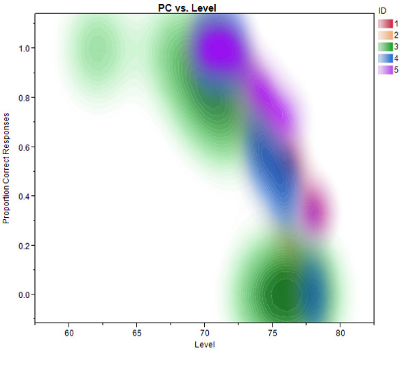
P.S. For those of you wondering about the data presented in this blog post – I made this plot in the Graph Builder platform of JMP. Graph Builder makes it very easy to drag and drop variables and change the visualization type that is displayed. In this case, I’ve chosen a Contour Plot for this data set.
What we are looking at is an experiment where I collected how well subjects were able to repeat back sentences played over headphones at the same time a masking background noise was played at various levels. I was interested in collecting a threshold for a specific level of performance – in this case, that signal-to-noise ratio (fixed level of the speech – the level of the noise) required to get 3/5 keywords correct 71% of the time. But in the process of collecting those thresholds, I also have access to the trial-by-trial data of how the subject arrived at that threshold (the noise is started at a low level and then gets progressive louder based on fixed decision rules – 2 correct answers and the noise increase, 1 incorrect answer and the noise decrease. These rules converge on the signal-to-noise ratio required for 71% correct criteria).
The individual trials for each subject shown in a different color gives me a nice sense of the slope of performance decline as the listening conditions get progressively harder. What you can see in the first figure is that when the noise level is low, the subject is performing close to 100% correct; as the noise level gets louder, performance at the task declines steeply to the point where the subject is unable to identify any words in the sentence correctly. Using the Contour Plot in Graph Builder is an excellent way to visualize this performance data across multiple subjects to see if I had any outliers, and also the concentration of trials at different noise levels.