Researchers commonly use complex laboratory methods to evaluate critical quality attributes (CQA) of drugs in development and throughout the product lifecycle. Instruments have validated ranges for obtaining data, and researchers often get results that are beyond the limits of detection (LOD). If you're a technical person running predictive models that include responses with limits on the range of values that can be obtained, this post is for you. JMP Pro now includes an easily deployed technique to appropriately deal with limits of detection within statistical models and reduce the risk for error.
What is the practical value of utilizing the new LOD controls in JMP Pro?
Let's consider an example: We are planning a set of experiments to determine the maximum amount of a solid impurity that can be extracted and measured with a laboratory method utilizing three inputs. The measurement method includes a lower detection limit of 1 unit. We've tried different techniques for dealing with LOD in the past, including using missing values, creating a value that is very small but not zero to allow for a logarithm to be used, imposing the limit for the observations affected by the LOD, and using the LOD control included in JMP Pro 16.
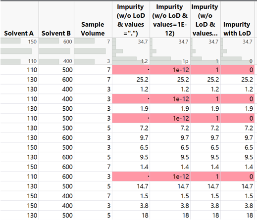
We use a generalized linear model with a log normal distribution utilizing forward selection to model the amount of impurity that can be extracted and measured. Running the model without LOD control results in predictions that are highly suspect to include significant error.
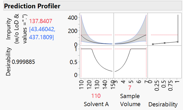
The maximized model using missing values provides an estimate of 137.8, which is hugely beyond the highest impurity amount of 34.7 realized in the experimentation. Note the extremely wide spread of the 95% confidence interval limits.
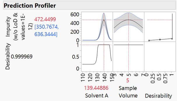
The maximized model using values that are close to zero provides the unrealistic estimate of 472.4.
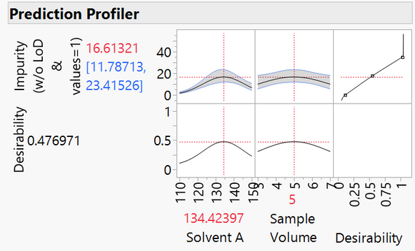
The maximized model using the 1-unit low limit seems to underestimate the optimum amount of impurity at 16.6, which is roughly half of the maximum amount realized during the experimentation.
We use LOD controls in the final model. The optimum amount of impurity that can be measured is estimated to be 36.7. Note that the realistic estimate comes from a model that includes all three method inputs. There are local maxima for each of the three method inputs, which makes sense to subject matter experts.
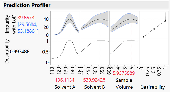
The comparison clearly illustrates how LOD controls mitigate error in prediction estimates for models. It is always a best practice to create confirmation runs in the space surrounding the amounts for the inputs identified as optimum.
What are limits of detection?
Instruments typically produce values from a matrix without an analyte, which are known as blank readings. A group of blank readings form a distribution of “noise” that is inherent with the measurement system. This “noise” is the random variability that you can expect from taking multiple readings of a homogenous sample tested by the instrument.
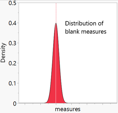
The limit of detection is the smallest concentration/quantity that is statistically different than a blank reading[1].
Smallest quantity = mean of blank measures + (confidence level x standard deviation of blank measures)
Using a 99% level of confidence, the limit of detection is the mean of the smallest signal that is roughly 3 standard deviations (blank) above the mean of the blanks.
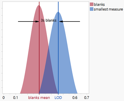
A limit of quantification is often utilized to mitigate a false negative result (that is, we assume the measure is outside of the limit when an actual measure is available).
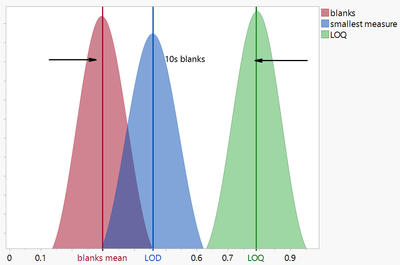
Some measurements have bi-lateral limits. Load cells that measure force typically have a zone of accuracy within bi-lateral limits.
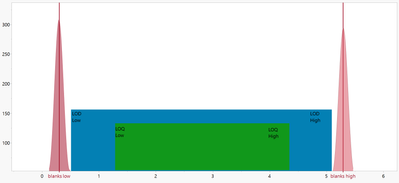
Scientists and engineers deal with many different types of limits of detection including: Instrument detection limit, method detection limit, limit of quantification, and practical quantification limit. Regardless of the type of limit used, it is up to the scientist or engineer to identify the cut-off values for censoring with LOD to meet the goals of experimentation.
Why do limits of detection affect model estimates?
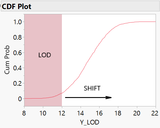
Parameter estimates are typically made with the cumulative distribution function (CDF). With limits present, the result is a shifted CDF and altered parameters. The plot below illustrates the effect of an LOD for a symmetric distribution.
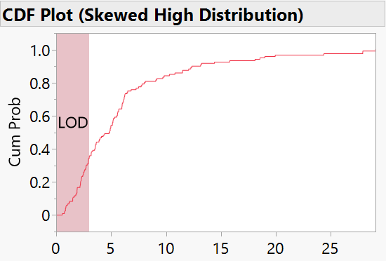
The shift of the CDF due to limits within measurements is especially profound for skewed distributions, which is seen below as a significant amount of potential data that is not included in the CDF that creates a big shift in parameters.
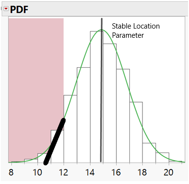
When we use limits of detection appropriately as censor values, estimates are made from the probability density function. The shape of the PDF mitigates the shift of the parameters since the missing portion can be Parameters are more accurate yielding realistic model estimates.
How can you utilize LOD controls in JMP Pro?
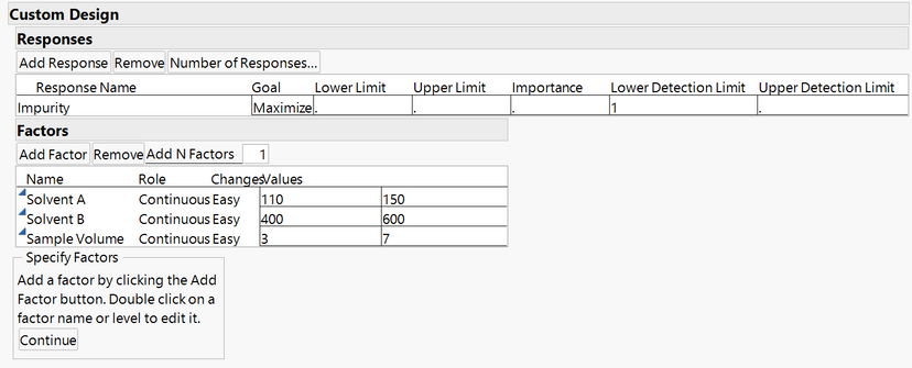
Let's consider a similar scenario: We are planning a set experiments to find out the maximum amount of a solid impurity that we can extract and measure using a laboratory method. We use the DOE> Custom Design menu option to set up the structure of the experiments. JMP 16 includes the ability to add detection limits as part of the design process as shown below.
Another way to set up LOD controls is to add them to the column properties.
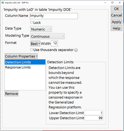
JMP Pro will automatically control for LOD without you needing to create additional columns required to censor appropriately for the limits within models.
Realize practical value by utilizing LOD controls
Use of this LOD controls in JMP Pro 16 yields significant improvements in the precision and accuracy of model estimates to enhance quality by design (QbD) efforts. Technical people now have a great new tool to deal with measurement methods that are known to have limits.
Reference
[1] IUPAC. Compendium of Chemical Terminology, 2nd ed. (the "Gold Book"). Compiled by A. D. McNaught and A. Wilkinson. Blackwell Scientific Publications, Oxford (1997). Online version (2019-) created by S. J. Chalk. ISBN 0-9678550-9-8. https://doi.org/10.1351/goldbook.