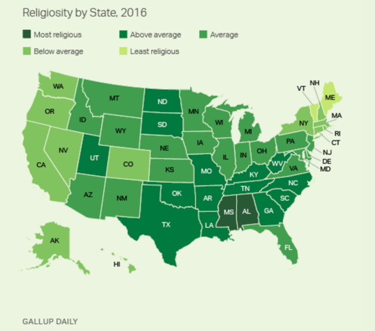
This map of religiosity from Gallup shows the percent of respondents who were classified as “very religious” in a 2016 poll. I noticed that many of the most rural states have high religiosity and the many urban states have low religiosity, and I wondered how much of the religiosity might be related to the ruralness of the population.
Getting the religiosity data from the Gallup article and Census Bureau urbanization data from Wikipedia was as simple and File > Internet Open in JMP. Now we can look at maps of both variables with similar color encodings. I'm defining ruralness as the inverse of the percent of urban population in the state.
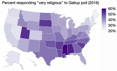
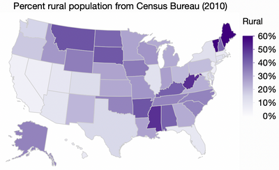
There is a lot of similarity but not as much as I imagined. A scatterplot makes the comparison more direct.
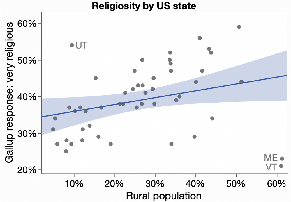
I added a regression line, and its confidence interval suggests the relationship is not very convincing since a flat line (which indicates no relationship) also goes within the confidence region. However, most of the dots appear to follow different linear trend, and a few outlier values on the edges are acting as leverage points and flattening the regression fit. If we think those states are categorically different, we can exclude them from the regression. For instance, the Gallup article notes that Utah is exceptional because of its large Mormon population.
“Robust” fitting techniques try to accommodate outliers without case-by-case consideration. One technique is to iteratively down-weight observations that are far from the line. That’s the method used by robust Loess. Other robust fitters in JMP include Huber, which reduces the outlier penalty, and Cauchy, which expects more extreme outliers.
Fit Cauchy within the Bivariate platform assumes that the error distribution follows a Cauchy distribution rather than a Normal distribution. The Cauchy distribution is nefarious in statistics because it does not have a well-defined mean or variance. It looks like a Normal distribution but has much fatter tails, which means it expects more of the data to be far away from the middle.

Nonetheless, it does have a central area where most of the distribution lies. Below is the result of a Cauchy-based linear fit on religiosity versus ruralness. In JMP, I saved the prediction formula and confidence bounds from Bivariate and plotted them in Graph Builder using the Line and Area elements. The line suggests there is at least a good subset of the data that follows a linear trend. The previously identified outliers are clearer, and a few more states that buck the linear trend stand out from the line.
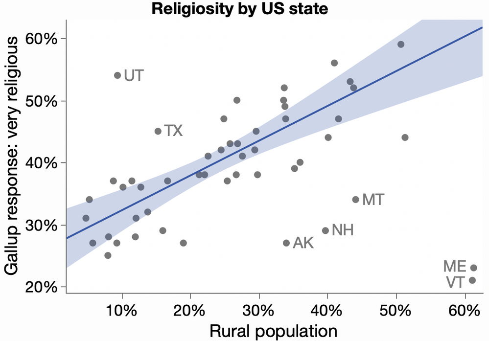
If some of the religiosity is indeed a function of ruralness, we can get a sense of how much is due to other factors by looking at the residuals. Let's bring it all back to a map to look for geographic patterns. Here’s a map of those residuals, which gives another perspective on the most and least religious states. For instance, Mississippi is no longer an extreme value, and Georgia and Florida look more like their Southern neighbors.
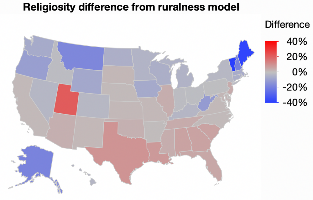
It’s worth emphasizing that the two variables come from different years and different sources, so don't read too much into the results. In particular, the ruralness of the Gallup participants may not match the overall ruralness of their state. Nonetheless, I thought the Cauchy fit shows a nice way to find a linear pattern among outliers.
Choropleth maps look simple, but they aggregate data within cultural boundaries over geography, and it’s good to keep in mind the underlying components.