- User Community
- :
- Blogs
- :
- JMP Blog
- :
- Be more confident in confidence intervals
We all need a little more confidence, right? Well…maybe there’s one area where we should have a little *less* confidence. Ironically, that area is our interpretation of confidence intervals.
First off, let’s talk about why confidence intervals are useful. When we do inferential statistics, we’re doing it because we don’t have all the information or data from our population. We’re making informed guesses, but we won’t always be exactly right. Like when we use statistics to see whether a sample of 200 students at your local college have a higher IQ than the general population. If we measured every single student, we wouldn’t need statistics. We’d have the truth about what the average IQ is and whether it’s higher than the population average of 100.
For example, you might guess that the average pour in your favorite brewery is 15.7 oz (with a standard deviation of about 0.51 oz) based on your careful – if not over the top – measurement of the mean volume of the 10 beers your friends consumed last night.
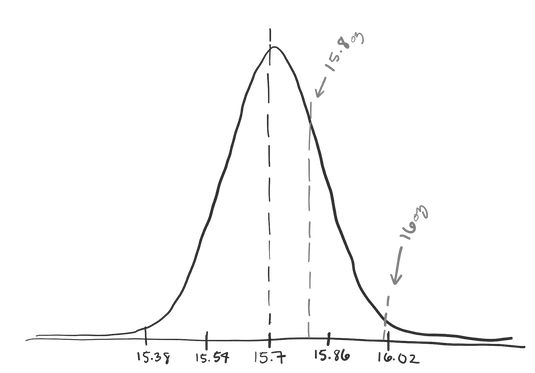
The bar claims that it pours 16 oz, so you might feel a tiny bit annoyed at the loss of 0.3 oz of your favorite Belgian ale.
But even though 15.7 oz is your best guess, it’s not likely that 15.7 is the *exact* population mean for beer volume. It would be more accurate to say that getting a mean of 15.7 oz makes you pretty confident that the population mean is *near* 15.7 oz.
This uncertainty – the whole “near” part – is something we often want to represent numerically. The way we do this in a Frequentist, Null Hypothesis Significance Testing (NHST) framework is with a confidence interval.
A confidence interval allows you to present a range of values instead of a single point estimate. You can think of this range as reasonable candidates for our population parameter (here, the mean) based on the data. This range is useful because it emphasizes the inherent uncertainty in our point estimates. Just like how you don’t necessarily expect babies to be born *on* their due date, but rather, around it.
But trying to do inference with confidence intervals? That can get a little bit tricky. Confidence intervals come paired with a confidence level, like 95% or 99% – though you could calculate a 90.273612% confidence interval if you really felt like it...although everyone would probably think you’re really weird. But once you have your confidence interval, what does it mean?
Sampling Distributions
Before we answer that, I want to take one tiny step back and talk about that Frequentist framework that I mentioned earlier.
Frequentists treat the population parameter as some true, unwavering value – and the samples of data we collect as random.
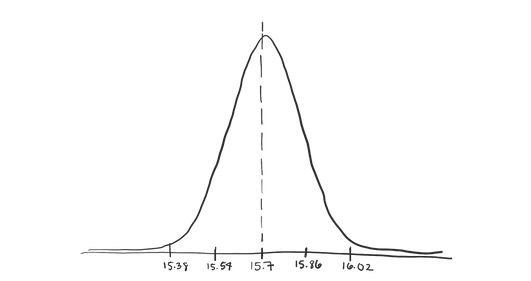
We could plot all the possible sample means that we could possibly get by calculating the average volume of 10 different beers poured at your local brewery. Since all we have is our sample data, this is our best guess at what that distribution might look like.
This is called a sampling distribution, short for sampling distribution of sample means, which is a bit of a mouthful. And as I mentioned, it’s a distribution that tells us how likely we are to get each mean value if we took a random sample of 10 beers from this brewery and calculated its mean.
And it’s a pretty good way to represent our uncertainty about whether 15.7 oz is *exactly* the population mean. Based on the data we have, 15.7 oz is the most likely value, and it’s the highest point on our distribution. But it’s also reasonable that we might get an average of 15.8. And relatively unlikely – but possible – that we’d get a mean volume of over 16 oz.
So if this distribution represents 100% of the possible means we expect to get, we can hedge our bets by using it to create a range of reasonable values.
Back to Confidence Intervals
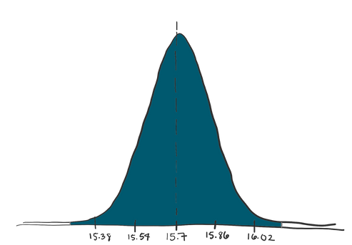
Let’s say we want to be *really* careful. We want our range to contain 99% of the values in our distribution. We could calculate where the middle 99% of the density of this distribution is.
We do this by using relying on the fact that the sampling distribution will be shaped like a t-distribution with n (the sample size) minus 1 degrees of freedom.
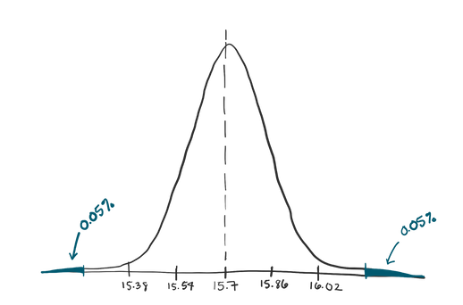
If we want the *middle* 99% of the distribution, that means we want 1% of the distribution to be outside our range, that is 0.5% on either side. So we can find out where the 0.5th and 99.5th percentile lie on this distribution.
A quick Google search or calculation will tell you that a t-value of -3.249836 represents the 0.5th percentile and a t-value of 3.249836 represents the 99.5th percentile. So anything between these two t-values is inside our 99% confidence interval.
But we don’t really want t-values ... we want our range to be in our regular units: ounces! Luckily, we can quickly convert them.
A t-value is the distance between two means (usually an observed mean and a baseline mean), divided by the standard error (which is just our sample standard deviation divided by the square root of n).
For example, if we wanted to know the t-value for getting a sample of 10 beers that had a mean volume of 16 ounces, if the true average were the 15.7 ounces, we can calculate that.
So, to convert *from* a t-value *to* ounces, we need to do this process backwards. We multiply by the standard error, and we add back the mean.
That means our confidence interval range goes from about 15.18 to 16.22oz.
OK, so we calculated a 99% confidence interval, and we know that it’s the range that contains 99% of the density of our sampling distribution ... but the next step is *interpreting* that interval ... which can be a little tricky.
Interpretation
This interval contains *most* of the values we think are reasonable based on the data we observed. So it *probably* contains the true population mean, right?
Well, probably. The 99% in a 99% confidence interval also tells you that if you calculated a BUNCH of different 99% confidence intervals using this exact procedure, about 99% of them will contain the true population mean.
But it’s pretty easy to take that true fact, and conflate it with the common misconception that a single 99% confidence interval has a 99% chance of containing the true population mean. That’s not true.
The “confidence” that we have is in the *process* of calculating confidence intervals...not in our specific confidence interval.
Example
And confidence intervals can be used for decision making as well. Say that you work at a beer factory. Maybe the same one that supplies the delicious brews at your favorite local brewery. And you have a machine that can measure the percentage of “soft” resins to “hard” resins in a batch of hops, the stuff that gives beer its distinct, musty flavor.
You want this value to be around 8%, so for every new shipment of hops, you take a few samples and record the percentage of “soft” resins. Then you calculate the 95% confidence interval for your “soft” resin percentage.
As long as that confidence interval contains 8%, you assume this batch is fine, since 8% is one of the population values we find “reasonable” based on our sample. So, you send it off to the factory.
If your confidence interval *doesn’t* contain 8%, you consider this batch of hops to be subpar, and you send it off to a farm to be used in animal feed.
If there were *never* a problem with your hops and the true percentage of “soft” resins was always 8%, 95% of the time, your confidence interval would contain 8%.
And 5% of the time it would not. This 5% is what we’d call a false positive – or Type I Error – since you’ve mistakenly flagged a perfectly good batch of hops as being subpar. But, the good news is that you’re in control of how often this happens.
This false positive rate will always be 100% minus your confidence level. So as a business, you can decide just how often you’re willing to mistakenly throw out good hops.
Essentially, you’re trading the financial loss of a feeding a few good batches of hops to the pigs for the ability to catch batches of hops that are *actually* bad.
Inference
Using the confidence interval for inference is pretty similar to doing a t-test on the same data.
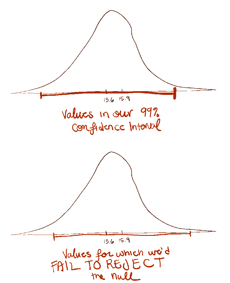
Our 99% confidence interval for the ounces of beer poured at your local brewery was 15.18 to 16.22 oz. Since 16 oz – the average that the brewery claims is true – is inside our confidence interval, we can’t claim to have evidence that they’re under-pouring. We still think 16 oz is a relatively "reasonable" value based on the data we observed.
And by "reasonable" we mean that it is within 3.25 standard errors from 15.7 oz. The 3.25 comes from finding the critical t-value for a 99% confidence interval. It marks the cutoffs for where 99% of the sampling distribution is, leaving only 0.5% of the distribution in either tail.
If a value is less than 3.25 standard errors away from 15.7 oz, then we consider it "reasonable."
And it turns out, if we are doing a t-test using alpha = 100%-confidence level (that is, p < 0.01), we are also testing whether two numbers are more than 3.25 standard errors apart. But this time, we're looking at whether our sample mean – 15.7 oz – is more than 3.25 standard errors away from our hypothesized mean – 16 oz. When something is more than 3.25 standard errors away from 16 oz (with n = 10), we reject the null hypothesis. If it's less than 3.25 standard errors away, we fail to reject the null hypothesis.
Since 16 oz was in our 99% confidence interval, we already know it's less than 3.25 standard errors away from 16 oz, and therefore a mean of 15.7 oz would *not* be significantly different from 16 oz at the p < 0.01 level.
In fact, any value inside your confidence interval is one that would *not* be significantly different from your sample mean when alpha = 100% - confidence level.
Confidence Intervals in JMP
Let's create a confidence interval for the heights of superheroes from a Kaggle data set (also see attached data table). You can use the Analyze>Distributions menu in JMP. Select Height, and add it to Y_columns. Select OK, and look for the red triangle next to your variable in the window that pops up. Select Confidence Interval from the menu, and choose your desired confidence level. Boom! You got a confidence level! The 95% confidence interval will display by default, but you can use the menu to select other confidence interval levels.
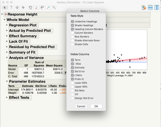
You can also create confidence intervals for your parameter estimates (like means, and regression slopes) from the Fit Model platform. Create your model using the Fit Model platform – like this regression model of superhero heights and weights – and scroll down to Parameter Estimates. Right-click on the table and select Lower 95% and Upper 95%. Your Parameter Estimates table now includes confidence intervals!
If you want to be even more efficient, you can also hold down Option + Right Click to reveal the settings panel for the table and check both boxes at once.
Now that you know a little bit more about confidence intervals, hopefully you can be more confident (oh, come on, you know I had to…) in their interpretation. Happy analyzing!
You must be a registered user to add a comment. If you've already registered, sign in. Otherwise, register and sign in.
- Subscribe to RSS Feed
- Mark as New
- Mark as Read
- Bookmark
- Subscribe
- Printer Friendly Page
- Report Inappropriate Content
- © 2025 JMP Statistical Discovery LLC. All Rights Reserved.
- Cookie Preferences
- Terms of Use
- Privacy Statement
- Contact Us


