The days are getting shorter, the kids are heading back to school, and NFL teams have started playing preseason games. That means it is time for some football predictive models.
A plethora of websites, magazines and “NFL experts” will come up with predictions for the coming NFL season. While some of the predictions will actually take historical data and statistics into account, many do not. If we have historical data, we should use it, so that is my plan. Before I get into how I built the model and what data I used, let’s look at the results.
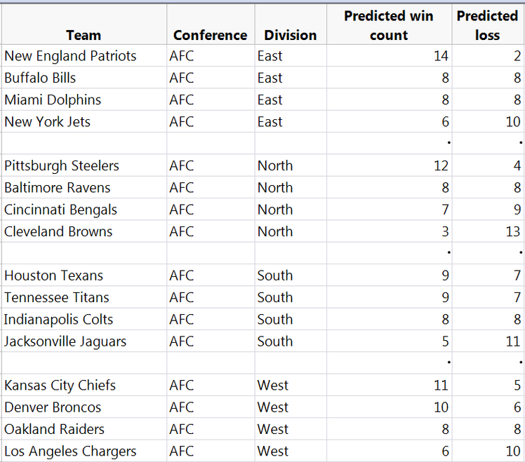
For the AFC projections, there's nothing too shocking. The team with the biggest change in win total from year to year is the Raiders, going from 12 wins last year to 8 this year. Every other team is within one or two wins of last year’s total.
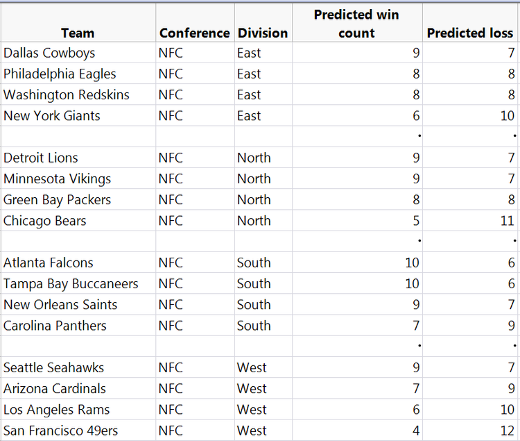
For the NFC, the results are a little bit more surprising, with the Cowboys and Giants losing four and five more games in 2017, respectively. Another thing I found a little surprising was that the Packers are projected to finish third in the NFC North. I was happy to see that that model did not have any wild projections, like the Browns winning 12 games or the Patriots winning three game. All in all, the model seemed very reasonable from a football perspective. Now let's get to how I built this model.
Building a model
My first goal was to get a bunch of historical data. I first tracked down historical payroll data (http://www.spotrac.com/nfl/cap/). I wanted to see if there was any magical combination of payroll that leads NFL teams to win. As the salary cap has increased from $120 million to $167 million, I used the fraction of the salary cap used for each position and position group.
Looking at historical salary data back to 2010, I found that there was very little correlation between teams winning and player pay. This was not too surprising since the NFL is full of bad contracts, which don’t necessary correlate to on-field performance. For example, the three highest-paid players in the NFL for the 2017 season are Joe Flacco, Carson Palmer and Kirk Cousins. While all three of these QBs might be above average, none of these guys is in the MVP discussion or has a place holder in Canton.
So I thought a better approach would be to try to predict the win difference from one year to the next based on salary and salary change of each position, position group. I also looked at some other factors like last year wins, points per game, yards per game and yards allowed per game. I had a total of 98 factors, so I needed to do some variable selection before running a full model. I used a bootstrap forest to perform my variable selection. The top 12 factors contributing to win differential are shown below in JMP.
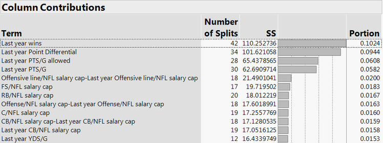
The top predictors are the wins a team had last year and the point differential a team had last year. While those factors might seem obvious, other factors that are important are less obvious. Factors I found intriguing were C pay, FS pay and RB pay. Typically center, free safety and running back are not viewed as critical positions. It might be that paying these positions highly has a detrimental effect on the team’s performance.
To determine the impact that each of these factors was having, I created a model. The top 11 factors are sorted by variable importance and shown in the Profiler below. I removed Last year’s PTS/G since that is completely confounded with point differential and points allowed.
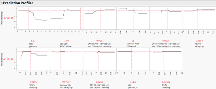
A few things stood out as unexpected:
- Spending more money on the offensive side of the ball leads to an improvement.
- Teams that allowed a lot of points last year improve more than teams that allowed less points.
- There is a distinct optimum range to pay your free safety.
Less surprising was that the most important factor is last year’s win total. It makes sense that bad teams will improve and good teams will get worse at some point. Good news for Browns fans! Not great news for the evil dynasty in New England.
For my final model to predict wins, I made an ensemble model. First, I created a validation column in JMP, so all of the models would be comparable. I saved the prediction formulas from bootstrap forest, boosted tree, neural network, and Generalized Regression models using the validation column. Then I took those model prediction formulas as factors in a neural network. Below is a comparison of all the models built.

Really cool! Look how much of an improvement I get from the ensemble model, with an R2 of over 0.86. Now let’s look at the actual vs. predicted plot.
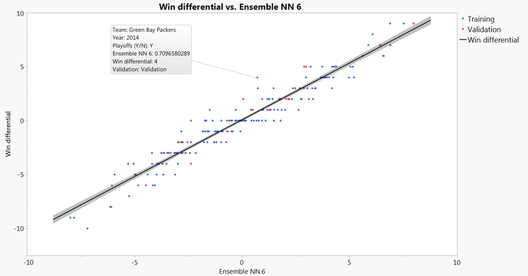
Not too bad. The worst miss for this model has been the 2014 Green Bay. The model predicted a win differential of approximately one, and the Packers actually won four more games.
In summary, I used historical salary and on-field performance data to predict the win differential for each team this year. The best performing model was an ensemble neural network model. Now let’s play some football and see how the model turns out!