- New to JMP? Let the Data Analysis Director guide you through selecting an analysis task, an analysis goal, and a data type. Available now in the JMP Marketplace!
- See how to install JMP Marketplace extensions to customize and enhance JMP.
JMP Blog
A blog for anyone curious about data visualization, design of experiments, statistics, predictive modeling, and more- JMP User Community
- :
- Blogs
- :
- JMP Blog
- :
- Applying machine learning: Will I beat my husband at pool on my birthday?
- Subscribe to RSS Feed
- Mark as New
- Mark as Read
- Bookmark
- Subscribe
- Printer Friendly Page
- Report Inappropriate Content

Two of my favorite machine learning algorithms, because they are easy to understand, are K Nearest Neighbors and Naïve Bayes. An algorithm doesn’t have to be complex to achieve good results, and for some problems these two algorithms perform quickly and accurately.
K Nearest Neighbors is pretty much exactly what it sounds like. The algorithm calculates which of the observations in the data set are the “K” nearest to the point you want to predict. Then the prediction is either the average of the response for those nearest points (if your response variable is continuous) or is the most frequent category (if your response variable is categorical). Typically, you fit a range of Ks and, using cross-validation, choose which K provides the best predictive performance.
I’m often asked why Naïve Bayes is called “Naïve.” The name comes from the fact that the key assumption that is made when using this algorithm is that all of the predictor variables are independent of each other. In many cases, that is a naïve assumption. Therefore, this method tends to perform better when that assumption is closer to true than if you have predictor variables that are highly correlated with one another. To make predictions, the probability of a category of the response (say, win or loss) given the observed predictor variables is calculated based on the probability of observing those values in the training data where that category is the response. Whichever category results in the higher calculated probability is the predicted category.
Let’s take a look at these two methods in action.
Who's Better?
My husband and I are avid pool players and play nearly every day when we get home from work. After a year or so of playing, we thought we were pretty evenly matched, with maybe me being slightly better. I said, “We can answer this question!”
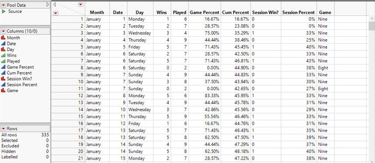
So beginning Jan. 1, 2018, we began tracking our results. I keep a spreadsheet (only because the computer in the game room at home doesn’t have JMP installed on it!) that tracks the month, day of the week, date, how many games I won, how many games we played, whether I won that gaming session, and which game of pool was played (8-ball or 9-ball). Because this was in a spreadsheet first, there are also columns calculating the overall game win percentage as well as session win percentage.
Thankfully, I can just drag my Excel file into my JMP Home Window, and the Excel Import Wizard works its magic to create a JMP data table. A few tweaks to make the Session Win? indicator a nominal variable and the number of games won and played to ordinal variables, and I’m ready to predict my next night of pool domination!
There are several options in the utility for how to create the validation column. If my response variable was highly unbalanced, which happens in cases where failures are uncommon or looking for fraudulent transactions, I would want to use the Stratified Random option to be sure I had data with both responses in the Training and Validation set. In this case, I know that all of my columns are balanced fairly well, so it’s unlikely that a category will be completely missing from my Training or Validation set. Therefore, I’ll just create my Validation Column using the Fixed Random option. I could set a seed for the random generation so I can reproduce this particular column again in the future, but I don’t think it’s necessary in this case.
Analysis Time!
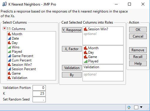
Now, validation column in hand, I can launch the K Nearest Neighbors platform in the Analyze > Predictive Modeling menu. Session Win? is my response variable and what I would like to predict, namely for my birthday, Saturday, Oct 13. [Note: I started writing this post before my birthday; read to the end to find out whether the predictions made herein were correct!] Month, Day, Game, and Played (the number of games played) are my factors. I don’t think Date will be helpful, mostly because each Month-Date combination occurs once (except for a few weekend days when we played multiple sessions). I’m also going to have the platform calculate the nearest neighbors up to 25 rather than the default 10.
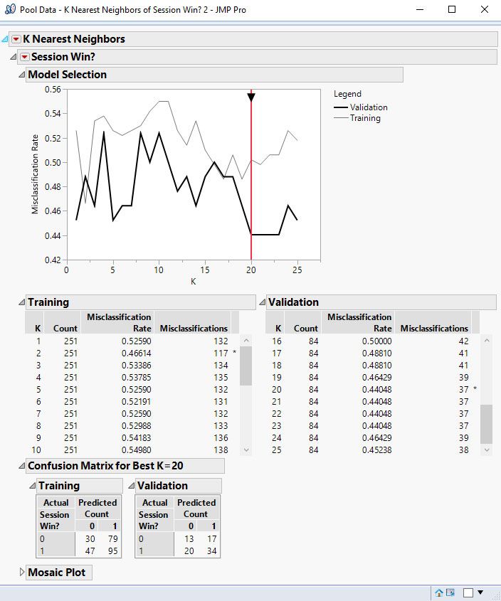
The Model Selection portion of the report traces the misclassification rate calculated on each of the Training and Validation sets for the models with 1 through 25 neighbors. The selection line is set at K = 20 – which has the smallest misclassification rate on the validation set. The table below shows that just over 44% of the observations in the validation set were misclassified. The Confusion Matrix shows that roughly the same number of observations that were actually wins or losses were misclassified. The Mosaic Plot gives a visual representation of the confusion matrix.
I’m going to save the prediction formula to the data table, so I can make my prediction about my birthday after I’ve fit these same data using Naïve Bayes.
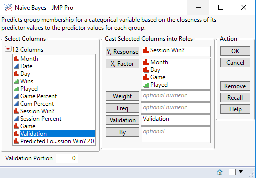
The first thing we notice is that the misclassification rate on the validation set is a bit smaller at just over 40%. The confusion matrix shows us that we’ve correctly classified seven more observations in the validation set with the Naïve Bayes model than the K Nearest Neighbors model. Finally, we have an ROC curve for each set. On the validation set, our area under the curve (another measure of the quality of the fit of the model) is 0.5676. While this isn’t great, it’s still better than random guessing, which would give us an AUC ≈ 0.5.
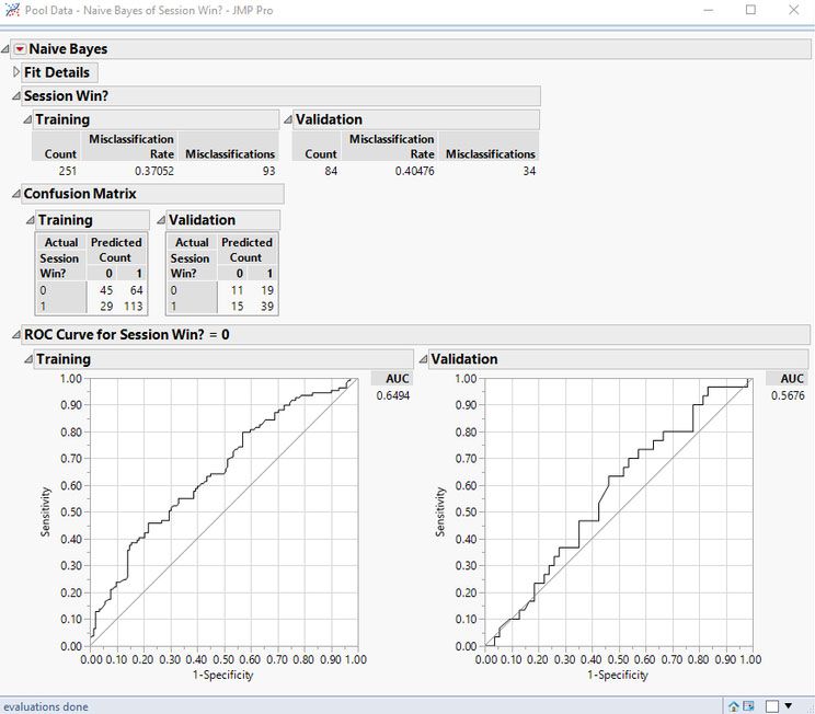
I’ll save the prediction formula to the data table again to make my prediction about my birthday pool performance.
Because we play a “best of 9” series when we play 9-ball, I don’t know ahead of time how many games we will play. Will I win quickly in a 5 – 0 rout? Or will it take all 9 games to determine a winner? I’ll add a row for each of the potential number of games played (5 through 9) and see what our models predict.
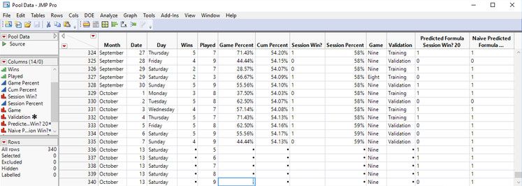
For this particular day, both models agree that I should be the winner unless the series goes to 9 games. In that case, K Nearest Neighbors predicts that I will lose. It’s going to be a happy birthday!
A few days later, my birthday arrived and armed with the knowledge that I will win, I entered the game room. An hour or so later, I exited, dejected, having lost three games to five. At least I got cake!
What Happened?
Things looked so good for me according to the models! How could I have lost? The Naïve Bayes model gives me a chance to look at the estimated probability of winning in addition to the ultimate prediction. It looks like I should have taken a look at those, too, rather than get my hopes up so high. I saved the probability formulas to the data table, and it becomes clear that while I was predicted to win, the highest probability was just under 75% and the lowest was just over 60%. That means my husband actually had a pretty good chance of winning. And by looking at just the final prediction, I misjudged my actual chances of a birthday win. I’ll take that as a word of caution to look at all of the information I have available before placing my bets next time!
![7 Data Table Pred Results.png Win probabilities. [Note: some data table columns hidden for space.]](/t5/image/serverpage/image-id/14493i1CB9FDD0FE63DFDD/image-dimensions/752x144?v=v2)
Parting Shot
A few final words on these models: Even the most advanced algorithms don’t perform well when the variables in the model aren’t very predictive of the response. We see that in action with these data and the high misclassification rates they have. As I stated earlier, this is not the fault of the algorithms, but a fault in the data I collected. Most models with reasonable predictors are much more successful than these were here. Maybe in 2019 I’ll add some more information to my data collecting and revisit these models.
In addition, pool is a sporting event where the human element plays a larger role in the outcome than many (maybe even most) usual applications of machine learning. You can see this play out nearly every weekend in the fall in collegiate and professional football games where an underdog pulls off an upset. This is sometimes referred to as “any given Sunday”. However, in the long term over many trials given these probabilities, I would win my bet; just like most of the time the favored football team wins, and the sports bettors make their money. And, in fact, if I look at subsequent days after my birthday, I did win about 60% of the time.
- © 2026 JMP Statistical Discovery LLC. All Rights Reserved.
- Terms of Use
- Privacy Statement
- Contact Us

You must be a registered user to add a comment. If you've already registered, sign in. Otherwise, register and sign in.