- Subscribe to RSS Feed
- Mark as New
- Mark as Read
- Bookmark
- Subscribe
- Printer Friendly Page
- Report Inappropriate Content
JMP Add-Ins
Download and share JMP add-ins- JMP User Community
- :
- File Exchange
- :
- JMP Add-Ins
- :
- Full Factorial Repeated Measures ANOVA Add-In
This Add-In generates the linear mixed-effects (random- and fixed-effect) model terms for one-way or full factorial repeated-measures designs involving a continuous response variable (categorical responses are not supported at this time)
Video Tutorials for Add-in:
One Factor: https://youtu.be/fh8jiFf2z-o
Factorial: https://youtu.be/py3-wvPYitM
Installation:
- Download factorial_repeated_measures.jmpaddin at the bottom of this page.
- Once downloaded, double-click the file to open in JMP.
- You will be prompted asking if you would like to install the add-in. Select Install.
- Under the Add-Ins menu, you will have a section for "Repeated Measures"
Factorial Designs:
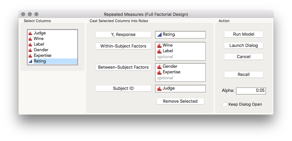
In repeated measures factorial designs, subjects are measured in each condition of the factorial combination of the within-subject factors, and are measured on only one level of between-subject factors. For example, subjects in a wine tasting experiment could taste and make ratings on several different wines, but are usually measured at one level of gender and expertise, as the levels of these factors are difficult to change in the time-course of an experiment. Full factorial designs involve a complete cross of factors. In the example experiment below, each subject tastes wine from 8 glasses, formed from the factorial combination of four different wines rated under the two conditions of Label ( four of the glasses were placed in front of bottles with expensive-looking labels, and four were placed in front of bottles with cheap-looking labels). The factorial cross of Expertise and Gender, the between-subject factors, involves measuring individuals in all four combinations (F/Expert, F/Novice, M/Expert, M/Novice). These factors are "between-subject" because no subject is measured at more than one level of the factors of expertise and gender.
Model Estimation
This add-in generates a linear mixed-effects model analysis. With no missing data, this analysis produces estimates and tests that are identical to a univariate, general linear model repeated-measures analysis assuming compound symmetry. However, mixed-models estimate model terms differently so estimates will be different (and potentially better) in the presence of missing data; univariate GLM repeated-measures analysis requires complete data, and subjects with missing cells are eliminated, whereas mixed-models can tolerate missing data without eliminating an entire subject from the analysis. Missing data (that isn't missing at random) can bias model estimates, so be sure to investigate the cause of missing data before interpreting the results of any model.
Usage:
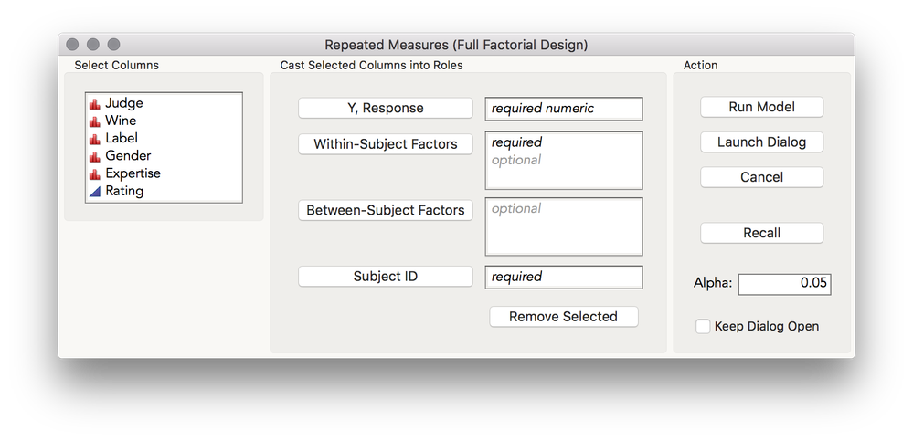
Cast columns into the appropriate role and click "Run Model," or click "Launch Dialog" to proceed to the Fit Model dialog to make changes to the model before running. To keep dialog box open after running, check the box for "Keep Dialog Open."
Note: For these models, "Subject ID" should have a Nominal modeling type; this add-in will automatically set the modeling type to Nominal if it is not already.
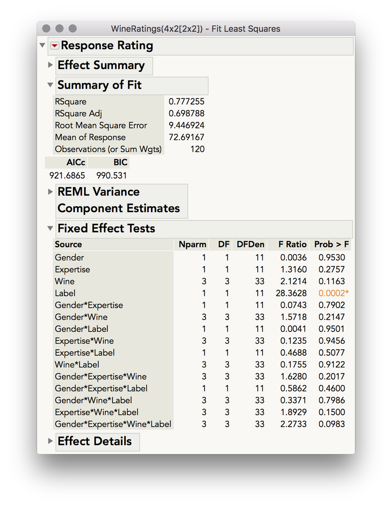
Model terms are generated, and an Fit Model output is launched with Summary of Fit details and Information Criteria, REML Variance Component Estimates, Fixed Effect Tests, and Effect Details.
| Model |
|---|
|
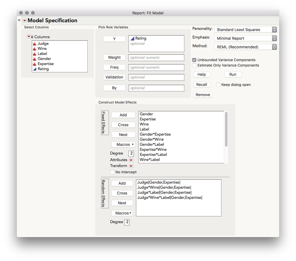
Effects( :Gender, :Expertise, :Wine, :Label, :Gender * :Expertise, :Gender * :Wine, :Gender * :Label, :Expertise * :Wine, :Expertise * :Label, :Wine * :Label, :Gender * :Expertise * :Wine, :Gender * :Expertise * :Label, :Gender * :Wine * :Label, :Expertise * :Wine * :Label, :Gender * :Expertise * :Wine * :Label ), Random Effects( :Judge[:Gender, :Expertise], :Judge * :Wine[:Gender, :Expertise], :Judge * :Label[:Gender, :Expertise], :Judge * :Wine * :Label[:Gender, :Expertise] ), |
Many options are available under the top-most Red Triangle, including additional regression reports, parameter estimates, diagnostic plots and saving residuals, leverage pairs, etc.
Plots, Means, and Tests
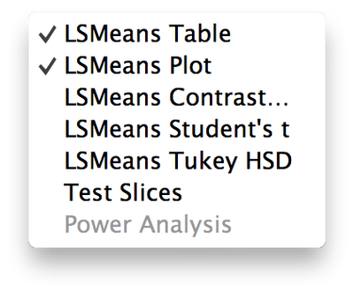
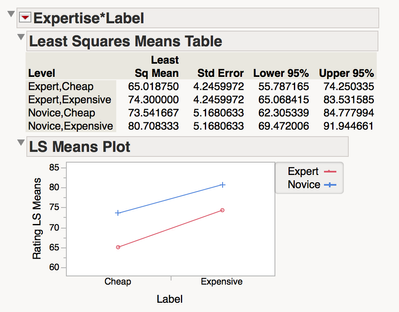
Expand Effect Details to generate plots for individual factors and interactions, and to perform tests on the cell means using all pairwise T-tests, Tukey HSD, and linear contrasts.
To interatively profile the model, select the top-most Red Triangle > Factor Profiling > Profiler
Modify and View Model
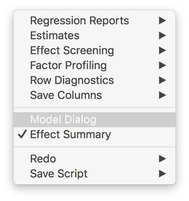
Select the top-most Red Triangle, and select Model Dialog to see the model specification and to make changes to the model.
Data format
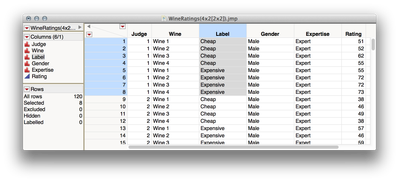
This add-in requires that data be in tall, or long format. This is when repeated observations from a subject are represented across rows, rather than across columns (see below).
If you need to restructure wide data, use Tables > Stack, and cast the columns with repeated observations in to the Stack Columns section. For factorial designs you will need to separate out the factor levels of each factor. By using Col > Recode this can be done quickly.
Additional Details:
- This add-in generates terms with the following algorithm:
- Full factorial of all fixed-effect factors (all within- and between-subject factors)
- Full factorial of only within-subject factors and subject-factor (with redundant terms removed)
- All terms involving subject are marked as random effects
- If between subject factors are present, all terms involving subjects are marked as nested in all between-subject factors
- If there are replicates of every cell (each subject was in each condition more than once) the highest order interaction with subjects is estimable. If there are not replicates, this highest order interaction is confounded with the residual (it IS the residual), and will be automatically removed.
- Models are limited to up to 5 within-subject factors, and up to 5 between-subject factors. If you regularly use models with more than 5 within-subject or 5 between-subject factors, please let me know.
Additional Videos:
I have a two sets of videos with more detail here that might be useful if you are going to us this add-in.
Module 2:8 - One Factor Repeated Measures
Module 2:9 - Factorial Repeated Measures
I hope this helps with your repeated measures analyses!
Update History:
v0.09: Added "Launch Dialog" button
v0.08: Added "Recall" button and "Keep Dialog Open" checkbox.
I am going to download and try this add-in, but I hope you can help with my question below anyway. I put this situation on the JMP User community post about 5 weeks ago but no suggestions so far. Where should I put it?
My data set consists of the questionnaire responses of several hundred teachers.
about one third are elementary, middle school, and secondary
they each rated the importance of 15 items on a scale of 0-3
(i am comfortable treating these ratings as interval level data; or ordinal is OK if that works)
I visualize this as a repeated measures ANOVA (between variable = teacher level; repeated variable = 15 ratings) with follow-up tests
But I have little interest in main effects: either repeated ratings (combining any particular item's scores across 3 teacher levels makes no sense), or across teacher levels (the items do not go together; each is stand-alone, so total score is of no interest)
instead, my questions are these:
1-for the group of elementary teachers, which of the 15 items are rated significantly higher than other items?
2- same for question middle school teachers
3- same question for high school teachers
4-does one of the 3 teacher groups rate item 1 significantly different than the other two groups?
5- same question for items 2—15
(I realize i am going to have to slice up alpha pretty thin to protect against inflation)
my first thought was ANOVA for repeated measures with followup tests, and just ignore the main effects to get to the followup tests.
but the Mauchly’s sphericity test was significant, seemingly (?) indicating the need for a MANOVA with followup tests. If so, how do I perform followup mean comparisons after a MANOVA in JMP?
Alternatively, should I be looking at a different analysis, since I am not interested in the main effects?
Hi dacullin,
Sorry for missing your message until now. Let me tackle each of your questions
Overall, your questions seem appropriate to analyze in the context of a repeated measures ANOVA (or a mixed model, which is what this add-in does), even if you don't have an interest in the main effects or interactions. There are a few things to consider though :
a) with a 0 - 3 scale you don't have much reason to think the population scores are normally distributed, so you might worry a little bit about that assumption of the model. However, you said you have several hundred teachers, so the central limit theorem is going to help you out in this regard.
b) it's probably the case that your covariances among questions differ -- some question answers will likely relate more strongly to others. In essence, this is what your Mauchly’s sphericity test was indicating -- a violation to that assumption. This does pose a little bit of a problem for followup tests, since some may be conservative and others anti-conservative. Analyzing subsets of your data can reduce a little of this worry since you are making assumptions about fewer covariances. If you are using JMP Pro, these tests can be run with unstructured covariances, but let's not go there just yet.
c) For the first three questions it sounds like you don't care about comparing item responses from teachers at different levels, so it might make sense to run these analysis separately for each teacher level (in this way, you wouldn't be including teacher level as a between-subject factor). An easy way to do this is using the data filter (Rows > Data Filter), and exclude all but the group of teachers you want look at. The add-in, as I have written it, does not include the option to use a By Variable, which would be the most direct way of doing this normally. I will add this to the list of features I want to add to this add-in.
- Alternatively, you can set up this analysis using Analyze > Fit Model, which does allow the use of a By Variable, by doing the following (assuming you have your data stacked as is illustrated in the add-in description above)
- Analyze > Fit Model
- Response as Y
- Subject ID as your first factor, select it in the model effects section, click "Attributes" then select "Random" - this will mark your Subject ID as a random effect so JMP knows how to correctly model it
- Add your Test Question factor to the model effects section
- Add Teacher Level as a BY variable
- This will return three separate Fit model outputs, one for each teacher level. From there you can do the following below:
Questions 1, 2, 3) After running the model using this add-in (after using the data filter to include only one group of teachers) you can expand the Effect Details section, which will show the source for Test Item. If you have used Fit Model with a By Variable you will see the Test Item source on the right-hand side of the output (which is the default placement, unless you changed the "Emphasis" in Fit model to "Minimal report," which is my preference and the one that the add-in above will default to.
After you found the section for your Test Item source, click the Red Triangle next to the name and you will get several options for performing pairwise tests. Given that you're interested in testing all possible combinations within the factor of items (which will be a lot of tests) I would recommend using the Tukey HSD option, which will control your family-wise error rate across all the tests within a given factor. The connecting letters report is a great way to look at the differences, or if you would like the adjusted p-values, you can click the Red Triangle in the Tukey HSD report, and select Ordered Differences Report.
4, 5) These tests require that you have teachers in the same model as items, so I would run a full model with teacher level as the between subject variable, and item as a within subject variable. My add-in helps with setting up that model, but if you're familiar with mixed models you can also do this through the Fit Model dialog directly. Once you have the model report, expand the effect details section and find the source for the interaction. In there you can use "Test Slices," which will perform contrast slices: a test for one of the factors at a single level of another factor. For example, you will get a slice labeled "Item 1" (or whatever that first item's label is) which will be a test of whether there is evidence that teachers differ in their responses for just Item 1. You will get those for all items. These seem like the most important tests for you, essentially one-way ANOVAs for the "effect" of teacher level at each level of item. With test slices you will also get a slice labeled "High School Teachers" (or whatever you have labeled that level) which is a test of whether there is evidence, overall, that High School teachers give different ratings for those items. These latter slices are probably of less use for you, especially since you will have looked at item differences in the previous models separately for each level of teacher.
If you would like to be most conservative for these tests of teacher level for each item, you could perform the same series of steps I suggested above for filtering your data, or using a By variable. This will mean you are setting up 15 different models, one for each item, with the single factor of teacher level. Once you have each model, you would then run the Tukey HSD test, giving you the connecting letters reports, or the ordered differences with p-values if you request them. This might actually be a better course of action since you wouldn't have to assert anything about the covariances among items since you're subsetting your data to include only one item at a time.
If you are going to us this add-in, I have a two sets of videos with more detail here:
Module 2:8 - One Factor Repeated Measures
Module 2:9 - Factorial Repeated Measures
I hope this helps!
Hi Julian,
I've been using your addon extensively, and really like it. My one major complaint is that it doesn't have a recall button like many of the other platforms. Any chance that could be added?
Thanks!
Hi benson.munyan,
Yes, that's a great suggestion! I've added it to the list of improvements for the next version. I'll also add a check-box to "Keep Dialog Open," which is something I often do in Fit Model when trying out different models.
Julian
Hello,
I have just downloaded this Add-In and it looks great, but I am used to doing the analysis in the traditional JMP fit model. I am wondering if you could help me with the layout with my variables and experiment:
I have an experiment where our subjects (SUBJECTS) 3 treatments (TRT), each analyzed over 2 hours time (TIME), and several response variables were recorded (core temperature, heart rate, and skin temperature).
I am wanting to look at the repeated measures (treatment x time) and look specifically if there are any differences between the TRTs for each time point.
Let me know your thoughts!!!
Hi jxa014,
Sure, I'd be happy to give some guidance here! Is your datatable structured in the format I showed above (long or tall format, with repeated observations for a subject across rows)? If not, you will need to stack your data using Tables > Stack. Let me know if you need to do this and I can give more specific advice. It would also be helpful if you included an example of your dataset (even just a few rows worth) so I can advice you better.
If your data are in the right format, setting up the analysis should be straightforward: place your subjects variable (whatever uniquely identifies subjects) in the Subject ID section, place TIME in the Within-Subject Factor section (since you have repeated observations for subjects at different times). TRT could be within-subject or between-subject depending on your methodology. If you measured each subject under all three treatments, TRT should go in the within-subject section. If you assigned each subject to just one of the three treatments then TRT should go in the between-subject factor section.
Once you run the model you will receive the usual statistical output. If you're most interested in the time x treatment interaction you can find details on statisical significance in the Fixed Effect Test table, and under the Effect Details you can find the LSmeans and run follow-up comparisons.
I hope this helps!
Julian,
That was perfect. Thank you so much. I ran the analysis for one of the response variables and here was the result:
Fixed Effect Tests
Source Nparm DF DFDen F Ratio Prob > F
Trial 2 2 6.006 2.6589 0.1489
Time 1 1 2.938 389.5700 0.0003
Trial*Time 2 2 5.904 5.5986 0.0433
Now do I do follow tests on the trial x time interaction?
Hi jxa014,
You can perform follow-up comparisons by expanding the Effect Details section, and then using the red triangles next to each source in your model. It seems as though you're most interested in making comparisons among the treatments at different time points, which means you will look to the trial x time section, and then use one of the options there. I have some videos that demonstrate some of these follow-up options. These videos discuss a non-repeated measures factorial model, but the principals are identical.
Overview of simple pairwise comparisons in Fit Model:
Pairwise Comparisons in JMP with Fit Model (Module 2 3 4) - YouTube
General factorial anova:
Factorial ANOVA (4x4) Full Analysis (Module 2 5 10) - YouTube
Testing slices (which I think you might be especially interested in)
Testing Slices in Factorial Designs (Module 2 5 11) - YouTube
Those videos are part of video series of mine, Significantly Statistical Methods in Science, and you can find the entire set of modules here:
Significantly Statistical Methods in Science Playlist
Hope this helps!
Thanks Julian.
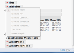
Yes, you are correct. I am trying to look at the differences between the time points per treatment. However, when click on the red triangle of the trial*time box under effect details box to run the analysis, it seems none of the options are highlighted. I am able to run further analysis under the Trial and Subject boxes, individually. Please see the picture if that makes sense:
This will happen if either time, trial, or both are marked as continuous in your dataset. All should be marked as nominal for this add-in and type of analysis to estimate the mean, and difference in means among treatment, at the different time points.
By the way, is Trial an alias for Treatment or did you mean to have Treatment in your model rather than trial?
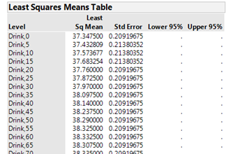
Yes, Trial and Treatments are interchangeable. In my model, there are 3 treatments/trials. I changed the trials and time to both nominal. Is it normal for the output to not give the upper and lower 95% CI when you do this change?
If you are missing those confidence intervals I suspect you also received other errors when trying to fit the model. From the number of levels you have for Time I suspect you don't have enough degrees of freedom to fit the model using time as nominal-- I expected you had measured individuals on far fewer time points. Given the number of levels you have it seems you would be better off modeling time as a continuous effect -- that is, estimating a slope between Y and time for each condition rather than means for Y at each time point for each condition (which is what treating time as nominal is doing, and is thus expensive in terms of parameters estimated). This is not something my add-in is built to do -- the model you're trying to fit is one in which you're nesting random coefficients, something you can do with the dedicated Mixed Model personality in Fit Model in JMP Pro. Here's the documentation page on that:
Launch the Mixed Model Personality
Sorry my add-in wasn't able to help you with this analysis!
Julian
Julian,
I think you are right on multiple accounts. The time in my study is continuous (0-120min; 5 min increments) as well as the df. I am doing preliminary analysis and we only have an n of 4, so more subjects are needed. However, now I know the process for the 2 way anova plug in.
Thanks for your help!
Hi Benson,
I wanted to let you know that I've added "Recall" and "Keep Dialog Open" options to the newest version of this add-in. I hope this helps!
Julian
Great Add Add-In! Saves a lot of time compared with manually entering the the same model in the Fit Model dialog.
The only problem so far is with column names that contain odd characters like "%", "(" or "/". I get error message and the log reads
"Cannot find item "Response Cs137/kg dw" in outline context {"Response Cs137/kg dw"}
Name Unresolved: Cs137 in access or evaluation of 'Cs137' , :Cs137/*###*/Exception in platform launch"
But despite this a report is generated with identical estimates but with a different set of outline boxes (fit model default?).
(I use JMP 12.2 for Mac)
Thank you for the feedback, MS! I really should make this more robust to special characters, and it sounds like I've done that in some places but not others!
- Mark as Read
- Mark as New
- Bookmark
- Get Direct Link
- Report Inappropriate Content
My study design is 2 x 2 x 3 x 3. The first three factors (2x2x3) were within-participants, and the third (with 3 levels) was between. When using the add-in, the report says that I have “Lost DFs,” which I am assuming means degrees of freedom, under the section Fixed Effects Test. Also, it isn't giving any other output under Fixed Effects Test Can anyone let me know why this is coming up?
Hi Julian,
I would like to ask for help since I have difficulties in understanding three types of strategies applied to study the repeated measures. In my study, all of them give different results. These models include the following:
1) Full factorial mixed ANOVA add-in
2) Mixed model analysis by using the fit model and random subject in the attribute section: https://community.jmp.com/t5/JMP-Academic-Knowledge-Base/Mixed-Model-Analysis-OPG/ta-p/21747
3) Mixed model personality with Pro
My design includes 16 advertising in 4 categories seen by 2 groups of consumers. I study their differences in cognitive engagement.
1) for a first model, I use cognitive engagement as a dependent, consumer group as between, advertising category as within, and subject ID as a random effect.
2) My random intercept is the Subject ID, my dependent is cognitive engagement, I model consumer category, ad category, and their interaction.
3) I do not have Pro version. Is there any difference between doing a mixed model analysis as in the second case or using the mixed model?
Thank you so much. I really appreciate your help.
Cheers
Dalia
Hi @Dalia,
I just responded to your private message but thought others reading these comments might be interested in the response, so I'm pasting it here. I hope this helps clarify some things!
---
Hopefully I can help a little bit with this! Mixed models can certainly be complicated, especially since there sometimes isn't a single "correct" model for a given situation. This add-in will fit a 'maximal model,' and by that I mean it will fit all the possible interactions between your subjects (the random effect) and your fixed effects (actual factors in your experiment). If you're not too familiar with mixed models, that's probably not terribly helpful. What this means, generally, is that you're estimating more parameters in a full maximal model than a simplified model in which you're estimating just a random intercept for each subject. In the simplest model, with just the random intercept (just the term for subject marked as random, but no interactions between the subject variable and other variables), you are asserting that subjects differ only in their average rating from one another--that they will react the same to your manipulations (and this is the model you ran by following the pdf in the learning library). In this model, any variation you observe between different subjects in how they respond to stimuli is classified as pure error, rather than real differences in how people react to the stimuli. This is generally not realistic; however, this kind of model uses far fewer degrees of freedom, and thus, you have more DF for error, which in general means more power.
So what's better? I like using my wine example for this -- in the example for the add-in, the model will fit an interaction betweens subjects and type of wine (red or white). This is helpful because some people like red wine more than white, and some like white more than red. Since there is a parameter in the model that can account for that variation across people, differences observed in average reaction to white and red wines isn't construed as pure error, but as systematic variation across people. With a large sample size, being able to distinguish between that systematic error and pure error would lead to more power. With a small sample, it's likely that one would miss effects by fitting all the extra interactions, unless that is, the interactions are truly quite large (e.g., you have a group of people who differ widely in their preferences for wine).
So, this is all to say, in general, for human subjects, I tend to think these interactions between the random effect (our subjects) and the fixed factors are worth estimating since it's hard to believe that people, unlike machines, will react the same to manipulations. If you have small samples, it's sometimes better to work with a reduced model with just some of the random slopes (interactions with subjects). You can get a sense of how much variation the random slopes account for by looking under the "REML Variance Components" section. If the interactions with subject account for a large percent of the total variation they're probably useful, otherwise, some would argue you should remove them. Remember, you can always go to the red triangle at the top and select "Model Dialog," and then go into the random effects section to remove terms.
Hi Julian,
I would like your advise on how I should analyse my data using this analysis and if this analysis is suitable for my data.
I have hourly measurements of water temperature data for 5 months across 5 sites.
24 x 30 x 5 x 5 = 18000 data points.
I want to see if the water temperature is significantly different between sites at each month, and also if there is significant differences between sites overall i.e. site and site x month interaction.
My data is is long format, with following col names
1.Site
2.Day number (0-150)
2. Month (June-October)
3. hours (0-24)
4. Temperature(Response variable)
So I have been adding months and site in within subject factors.
I am a bit confused about which factor to put in Subject ID, if it should be Day number or hours ? I am not interested to see hourly or daily variations.
Also do you think I should use full-factorial repeated anova for my data or do you think I should rather do a mixed model by specifying a repeated structure (ex corAR1 etc) ?
Thank you so much.
Hi @tsingh,
I would be happy to give you some general thoughts, but time-series type data such as these are not my specialty so I think you might have better luck posting your question in the general JMP community. My intuition is that you probably shouldn't analyses these data with this Add-in. Now, that isn't to say that you couldn't -- Site could be your Subject ID, and Month a Within-subject effect, but you'll be ignoring all the autocorrelation among points close in time, and there is probably good reason to model the cyclical patterns of temperature both within and across days. Unless really could assert that measurements of temperature within a month for a given site were independent, I would go a different route! Again, the general community discussion board is a good place for this question -- I expect someone with some Time Series experience will have some advice to share.
Julian
@jules
Thank you for the quick reply, yes it seems I do have high temporal autocorrelations. I'll ask about this in general JMP community.
Hi Julian,
I would like to ask another question. Why do I get different estimates when I do a random intercept model on JMP and on SPSS? I can see that in JMP there are more degrees of freedom as compared to the output in SPSS. When it comes to the fixed effects, I get exactly the same result. Is that a problem actually, that two different software show the same statistical output, in terms of F value and p-value, but different estimates for fixed effects?
Thank you so much!
Cheers
Dalia
Hi Julian,
thanks again for this Add-on, it's super-useful, and so much easier to use than JMP's default way of doing things.
In case you're interested in suggestions for further improvements:
- adding options to test for the assumptions would be invaluable (especially when teaching using JMP, but also for everyday analyses)
- adding options to test for effect sizes would also be great, especially given that most journals, APA etc. ask for inclusion of effect sizes
- could this plug-in be expanded to also work on just between-subject effects? That it would likely become the main go-to for all my ANOVA needs ;)
Cheers & thanks!
Bernhard
Hi @bernhard,
Thank you for the suggestions! I'll add these to my list of future improvements and will be sure to let you know when a new release is available. By the way, for fully between-subjects designs, the standard Fit Model dialog works quite well: simply select all your factors in the columns list, then click the Red Triangle next to Macros, then Full Factorial (or Factorial Sorted) to automatically generate all the model effects.
Thanks Julian, looking forward to seeing what you'll cook up!
You're right, the "full factorial" macro is indeed useful
cheers
Bernhard
I'm trying to run an analysis with your add-in, and I get this error message:
Unrecognized Effect Option 2 times in access or evaluation of 'And' , :ID[:State] & /*###*/Random/*###*/
Any idea what it might mean?
Hi @jsheldon1,
I'm sorry to hear you're having trouble. It'll help if you can tell me more about what you're trying to do, and what your dataset is like. If you can attach a small piece of it that would be especially helpful. Without knowing more, the best guess I have is that you have special characters in one of your column names (this add-in isn't particularly robust to non-alphanumeric characters in column names). Could that be the problem?julian
Hi Julian,
I'm still a fan of this add-on, and was wondering what your timeline for the next iteration might be? E.g., currently, I end up using SPSS or another software to test for effect sizes as there doesn't seem to be an easy way to get those from JMP for within-subject or mixed-effect designs. Which is also a serious drawback when using JMP in teaching stats. Would be super-useful if this could be added into this plugin (or the "Calculate Effect Sizes" plugin could be extended to work for mixed and within-subject designs).
Cheers & thanks!
Bernhard
Dear @jules,
I have been using this Add in for a while now and it is very useful.
would it be possible to change the "nested" to "Cross" for the random coefficients? this would allow the usage of continuous "Between subjects factors". At the moment, when introducing a continuous "Between subjects factors" the fit model platform refuses to estimate the nested terms (and the model as a whole).
Many thanks to your innovative contributions.
ron
Dear @julian,
The F-ratio in the Fixed Effects Table that is generated using the Repeated Measures Addin is that based on Type II or Type III sum of squares? Seems like the F ratio are closer to calculated using Type II SS.
Recommended Articles
- © 2026 JMP Statistical Discovery LLC. All Rights Reserved.
- Terms of Use
- Privacy Statement
- Contact Us
