- New to JMP? Let the Data Analysis Director guide you through selecting an analysis task, an analysis goal, and a data type. Available now in the JMP Marketplace!
- See how to install JMP Marketplace extensions to customize and enhance JMP.
- Subscribe to RSS Feed
- Mark Topic as New
- Mark Topic as Read
- Float this Topic for Current User
- Bookmark
- Subscribe
- Mute
- Printer Friendly Page
Discussions
Solve problems, and share tips and tricks with other JMP users.- JMP User Community
- :
- Discussions
- :
- Re: non-linear fit
- Mark as New
- Bookmark
- Subscribe
- Mute
- Subscribe to RSS Feed
- Get Direct Link
- Report Inappropriate Content
non-linear fit
I am using JMP 8 to do a non-linear fit.
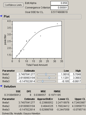
It generates a goal SSE value and a solution SSE value. I just wonder how to interpret these values. How to decide if the non-linear fit is a good one or not?
And is there any way to convert SSE to R square?
Attached is the output from the non-linear fit from JMP 8.
Thanks!
Accepted Solutions
- Mark as New
- Bookmark
- Subscribe
- Mute
- Subscribe to RSS Feed
- Get Direct Link
- Report Inappropriate Content
Re: non-linear fit
The SSE is the residual sum of squares of the best fit of the current model to the data. The Goal SSE for confidence limits is only used for estimating the confidence limits at current Alpha (there is a description in the JMP documentation in the "statistical details" of the nonliear chapter).
Although R2 alone should not be used to judge if a nonlinear model's fit is "good", it can be calculated from the SSE and raw data.
Try this JSL example (I only tested it in JMP 10, I don't remember if the the sample table came with JMP 8. If the path fails, try to open the table manually before running the remainder of the script)
// Example nonlinear fit
dt = Open( "$SAMPLE_DATA/Nonlinear Examples/US Population.jmp" );
nlin = dt << Nonlinear( Y( :pop ), X( :Name( "X-formula" ) ), Finish() );
// get SSE from report
SSE = Report( nlin )[Number Col Box( "SSE" )][1];
// Calculate total sum of squares (i.e. of distances from y mean)
SStot = Sum( ((Column( 2 ) << get as matrix) - Col Mean( Column( 2 ) )) ^ 2 );
// Calculate R2 and adjusted R2
R2 = 1 - SSE / SStot;
R2adj = 1 - (SSE / Report( nlin )[Number Col Box( "DFE" )][1]) / (SStot / Col Number( Column( 2 ) ) - 1);
// Update report with R2
Report( nlin )[Outline Box( "Solution" )] << prepend(
H List Box( Number Col Box( "R2", {R2} ), Number Col Box( "R2adj", {R2adj} ) )
);
- Mark as New
- Bookmark
- Subscribe
- Mute
- Subscribe to RSS Feed
- Get Direct Link
- Report Inappropriate Content
Re: non-linear fit
Thanks a lot!
Further question:A best fit shall have an SSE closest to 0, right? but normally we won't get 0 for the data we generate from experiment. So I just want to know if there is any criteria for the solution SSE to determine whether the current model generates a good non-linear fit or not.
Recommended Articles
- © 2026 JMP Statistical Discovery LLC. All Rights Reserved.
- Terms of Use
- Privacy Statement
- Contact Us
