- New to JMP? Let the Data Analysis Director guide you through selecting an analysis task, an analysis goal, and a data type. Available now in the JMP Marketplace!
- See how to install JMP Marketplace extensions to customize and enhance JMP.
- Subscribe to RSS Feed
- Mark Topic as New
- Mark Topic as Read
- Float this Topic for Current User
- Bookmark
- Subscribe
- Mute
- Printer Friendly Page
Discussions
Solve problems, and share tips and tricks with other JMP users.- JMP User Community
- :
- Discussions
- :
- Response Surface
- Mark as New
- Bookmark
- Subscribe
- Mute
- Subscribe to RSS Feed
- Get Direct Link
- Report Inappropriate Content
Response Surface
Dear JMP Experts,
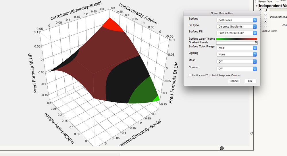
In the attached picture I created a surface plot with the graph-surface plot function. I created a color scheme with discrete color option. I am wondering what is the cut-off points for each of the colors? In another word, does the bright red mean the highest results? Does the dark red mean the stable region? How can I find explanations? Is there a way to show the cut off points for the independent variables by the color? Or does the color change mean anything at all?
Thank you a million!
- Mark as New
- Bookmark
- Subscribe
- Mute
- Subscribe to RSS Feed
- Get Direct Link
- Report Inappropriate Content
Re: Response Surface
The colour scheme you apply via 'Sheet Properties' is intended to help you visualise the shape of the surface, and there is a lot of flexibility. In the case of the 'Discrete Gradients' Fill Type, you can change the 'Surface Color Theme' (to one of the supplied themes, or one you have made up), define the number of 'Gradient Levels' (the number of colours), and 'spread' these colours over the range of the data, or over the range of the axis that's currently shown.
With some care, you should be able to 'see', where the boundaries are and (knowing what options you have applied), you could calculate them if you wanted to. For example, in this case, the highest boundary appears to be at about 170:
NamesDefaultToHere(1);
dt = Open("$SAMPLE_DATA/tiretread.jmp");
sp = dt << Surface Plot(
	Columns( :Pred Formula ABRASION, :ABRASION, :MODULUS ),
	Lock Z Scale( 1 ),
	Datapoints Choice( "Points" ),
	Z Grid Position( 130 ),
	Surface Color Theme( "Green to Black to Red" ),
	Surface Gradient Type( "Discrete Gradients" ),
	Formula( "Pred Formula ABRASION" ),
	Response( :ABRASION ),
	Surface Color Method( :Pred Formula ABRASION, "Solid", "Solid", "Solid" ),
	SetVariableAxis( :SILICA, Axis Data( {} ) ),
	SetVariableAxis( :SILANE, Axis Data( {} ) ),
	SetZAxis(
		Pred Formula ABRASION,
		Current Value( 130 ),
		Axis Data(
			{Min( 45.0232558139535 ), Max( 220 ), Inc( 50 ), Minor Ticks( 1 )}
		)
	),
	SetXVariable( :SILICA ),
	SetYVariable( :SILANE ),
	Iso Value( 0, 139.119238722664 ),
	Frame3D(
		Set Rotation( -90.8594176470491, -0.15205112334844, 58.1091217394078 )
	)
);
To answer a couple of your questions:
Beacsue of the options you have specified, then, 'yes' bright red shows the highest values.
Not sure if 'dark red' denotes a stable region, since that depends on how you want to define the latter. If you want to optimise a response, you might also consider using the Profilier, possibly with monte carlo simulation if you are concerned with robustness.
Recommended Articles
- © 2026 JMP Statistical Discovery LLC. All Rights Reserved.
- Terms of Use
- Privacy Statement
- Contact Us


