- New to JMP? Let the Data Analysis Director guide you through selecting an analysis task, an analysis goal, and a data type. Available now in the JMP Marketplace!
- See how to install JMP Marketplace extensions to customize and enhance JMP.
- Subscribe to RSS Feed
- Mark Topic as New
- Mark Topic as Read
- Float this Topic for Current User
- Bookmark
- Subscribe
- Mute
- Printer Friendly Page
Discussions
Solve problems, and share tips and tricks with other JMP users.- JMP User Community
- :
- Discussions
- :
- Peak of a probability distribution
- Mark as New
- Bookmark
- Subscribe
- Mute
- Subscribe to RSS Feed
- Get Direct Link
- Report Inappropriate Content
Peak of a probability distribution
Hi
I have a dataset which fits best to the Johnson Su distribution and I was wondering if there is a way to estimate the value of the peak of this distribution. It has just one peak, which is pretty different from the median or the mean. Calling this "mode" might be the best possible solution here but how do I estimate this point?
- Mark as New
- Bookmark
- Subscribe
- Mute
- Subscribe to RSS Feed
- Get Direct Link
- Report Inappropriate Content
Re: Peak of a probability distribution
Can the profile option be extended for data distribution that is grouped? For N groups, need to get the mode corresponding to distribution of each of the items in the group. Or should I subset by group everytime and then use the profiler option. I used the col groupby and then fitted but looks like it is giving a single value for entire dataset and not for each group member.
- Mark as New
- Bookmark
- Subscribe
- Mute
- Subscribe to RSS Feed
- Get Direct Link
- Report Inappropriate Content
Re: Peak of a probability distribution
Just to add on.
Mark's way is really the best way to get the peak value, but for a quick way to get an estimated value you can fit the curve then use the JMP Crosshairs tool found in the Tools menu or on your menu bar. Click the tool then put the crosshairs symbol on the spot you feel best represents the peak and a value will pop up. If you are using JMP 13 you will get a magnifier with the Crosshair tool that will help you get close.
HTH
- Mark as New
- Bookmark
- Subscribe
- Mute
- Subscribe to RSS Feed
- Get Direct Link
- Report Inappropriate Content
Re: Peak of a probability distribution
Mark's method is neat. Here's an alternative that uses the function directly:
NamesDefaultToHere(1);
ClearLog();

// Make some representative data
dt = NewTable("Johnson Su", NewColumn("Data", Numeric, Continuous, Formula(Random Johnson Su( 5, 2, 1, 1 ))));
dt << addRows(50);

// Fit the data
dist = dt << Distribution(Continuous Distribution( Column( :Data ), Fit Distribution( Johnson Su ) ));
// Get the fitted parameters
params = Report(dist)[NumberColBox(3)] << get;
gamma = params[1];	// Shape
delta = params[2];	// Shape
theta = params[3];	// Location
sigma = params[4];	// Scale

// http://www.mathwave.com/articles/johnson_su_distribution.html
//			f(x) = delta/(lambda * Sqrt(2*pi()) * Sqrt(z^2 + 1)) * exp( -1/2*(gamma + delta * ln(z + Sqrt(z^2+1)))^2 );
// 		where:
//			z = (x - eta)/lambda;
//		and:
//			delta > 0 lambda > 0
jsu = Expr(delta/(lambda * Sqrt(2*pi()) * Sqrt(z^2 + 1)) * exp( -1/2*(gamma + delta * ln(z + Sqrt(z^2+1)))^2 ) );
SubstituteInto(jsu, Expr(z), Expr((x - eta)/lambda));
// Use the fitted parameter values
// Note the change in parameter names! 'lambda' -> 'sigma' and 'eta' -> 'theta'
SubstituteInto(jsu,
	Expr(gamma), Eval(gamma),
	Expr(delta), Eval(delta),
	Expr(eta), Eval(theta),
	Expr(lambda), Eval(sigma)
);
// Get upper and lower bounds for the optimisation (either side of the (assumed) single peak)
vals = Column(dt, "Data") << getValues;
low = Quantile(0.25, vals);
high = Quantile(0.75, vals);
// Do the maximization
Maximize(jsu, {x(low, high)}, << Tolerance(10^-10), << showDetails(true));
Print(x);
('By eye' it seems to work, but no testing of course).
- Mark as New
- Bookmark
- Subscribe
- Mute
- Subscribe to RSS Feed
- Get Direct Link
- Report Inappropriate Content
Re: Peak of a probability distribution
One of the things that I love about JMP is that it often gives you many ways to solve a problem. All of the previous suggestions for finding the mode of the fitted Johnson SU density for the data are great, but here is one more option that uses the Profiler.
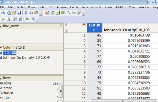
Once you have used Distribution to fit the Johnson Su distribution to your data, you can choose Save Density Formula from the Fitted Johnson Su menu. This saves the Johnson Su Density formula to a column in your data table.
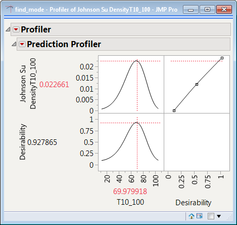
Next you can open the Profiler by choosing Graph>>Profiler. Cast your density formula as the Y, Prediction Formula and click OK. Next turn on the Desirability Functions from Prediction Profiler menu. After that you choose Maximize Desirability from the Prediction Profiler menu. This will find the mode (maximum) of your Johnson Su density for this data.
- Mark as New
- Bookmark
- Subscribe
- Mute
- Subscribe to RSS Feed
- Get Direct Link
- Report Inappropriate Content
Re: Peak of a probability distribution
Laura's method is neater! And far less error prone. It's always best to let JMP do the work for you if you can figure out a way.
- « Previous
-
- 1
- 2
- Next »
Recommended Articles
- © 2026 JMP Statistical Discovery LLC. All Rights Reserved.
- Terms of Use
- Privacy Statement
- Contact Us


