- New to JMP? Let the Data Analysis Director guide you through selecting an analysis task, an analysis goal, and a data type. Available now in the JMP Marketplace!
- See how to install JMP Marketplace extensions to customize and enhance JMP.
- Subscribe to RSS Feed
- Mark Topic as New
- Mark Topic as Read
- Float this Topic for Current User
- Bookmark
- Subscribe
- Mute
- Printer Friendly Page
Discussions
Solve problems, and share tips and tricks with other JMP users.- JMP User Community
- :
- Discussions
- :
- Re: Path analysis in JMP 16 Pro
- Mark as New
- Bookmark
- Subscribe
- Mute
- Subscribe to RSS Feed
- Get Direct Link
- Report Inappropriate Content
Path analysis in JMP 16 Pro
I have a data set of 768 rows of data taken over 32 months from plots with different ground vegetation and plant genotypes. Climate data (T, RH, and Rain) were collected during the same period from a nearby weather station. I have density estimated of aphids and occurrence data for ants and generalist predators. I would like to use path analysis in JMP to explore how the exogenous variable of climate affect aphid and ant predator occurrence on plants, and how ant and predator occurrences affect aphid densities on plants. I have been exploring the use of structural equation model feature of JMP 16 Pro to build the appropriate models, but I am still not confident of how to choose the appropriate models by parsimony while maintaining an appropriate fit. I have built the following model with 26 parameters
T, RH, and rainfall unidirectional effect on aphids
Ants and predator covarying with aphids
T covarying with RH
RH covarying with Rainfall
I get high CIF nearly 1 and RMSEA near zero
The output seems to be ok, but R2 of the endogenous variables - aphids, ants, and predators are quite low.
I tried the same analysis on a summary of the data - down to a sample size of 64. This gives me a lower CIF and higher RMSEA (i.e., poorer fit) but much R2 of each of the three endogenous variables.
My questions are:
1. is it ok to work with a summary of means rather than original data (sample size declines but no parameters is unchanged)
2. Is R2 of the endogenous variables important, compared with CIF and RMSEA
3. How can I justify reducing the number of parameters in the model but taking out variables and/or reducing the pairing of variables.
I look forward to interactions with interested members of JMP community to clarify my questions and hopefully get useful feedback to make sure I use the correct approach in analyzing my dataset.
Thank you
Rick
- Mark as New
- Bookmark
- Subscribe
- Mute
- Subscribe to RSS Feed
- Get Direct Link
- Report Inappropriate Content
Re: Path analysis in JMP 16 Pro
Hi Rick,
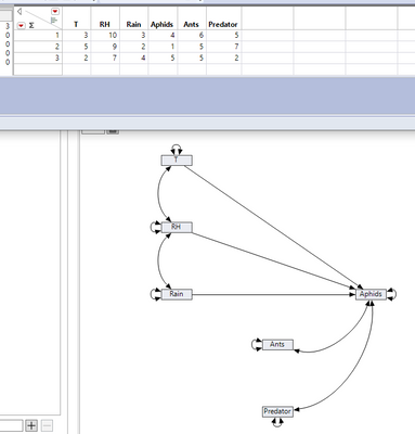
Great to hear you're exploring the use of structural equation models with your data! I made up 3 rows of data to gain clarity on the model you're fitting. Based on the description of effects in your post, I have the following path diagram:
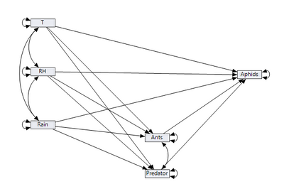
Is this similar to the model you're fitting? If so, I think there are some specification issues that might help. From your description of the problem in the first paragraph, I suspect a more appropriate model might look like this one:
However, I'm not sure I understand how time is represented in your data. Do you have 32 repeated measures for each of these variables (1 measure per month)? If so, are your data in "wide" or "long" format? SEM requires "wide" format. For example, you might have Rain_1, Rain_2, ... , Rain_32 for the repeated measurements of rain. You might consider watching the video on this link, which describes how to model longitudinal data in SEM:
To answer your specific questions:
1. Yes, it's fine, but the research questions change accordingly. If you took averages across all the repeated measures, then you're no longer able to examine time-sequential effects, which is often of interest when you have data taken over time.
2. CFI and RMSEA give you a sense of how well your model fits the data. This is of key importance because you only want to interpret results from models that fit well. Once you know your model fits the data, then you interpret the results, including the R2 of endogenous variables.
3. Reducing the number of parameters in a model should be done based on your desire to test specific hypotheses. For example, based on the second image I pasted, I might decide to fit two models: 1) a model just as I depicted, and 2) a model where I eliminate the unidirectional paths from climate (T, RH, Rain) to Aphids. I could then compare the two models to test the hypothesis of whether climate has a unique direct effect on Aphids above and beyond the indirect effect that goes through Ants and Predators.
HTH,
~Laura
- Mark as New
- Bookmark
- Subscribe
- Mute
- Subscribe to RSS Feed
- Get Direct Link
- Report Inappropriate Content
Re: Path analysis in JMP 16 Pro
Dear Laura, Thank you very much for the explanations and suggestions. The model I am trying to fit is a near full model (your second diagram) without Rain and T covarying, which I already determined that they don't covary. Ants and predators covary, which I kept in the model. The time element repeats over 32 months (data collected once a month) which I include as a column (not across). The design is a split plot design, in 3 replicate blocks. The main plot is ground cover (2), and the subplot is plant genotype (4), so total number of observations is 2 main plots x 4 subplots x 3 blocks x 32 months = 768 observations. Each observation is a mean of 4 plants of each genotype in each ground cover and block.
The exploratory analysis that I have already carried out showed that much of the relative humidity and temperature effects are indirect. The CFI and RMSE are respectively ~0.9 and <0.1.
You rightly pointed out that my approach is missing the sequential time element effect. How do I incorporate that into the model. Perhaps I don't need to worry about it. If I average across the 32 months, i would not have enough observations to fit my model. The repeated observations are allowing me to give the model sufficient number of observations - at least 10 per parameter. I would like to do a separate analysis overtime to determine how the predators and ants cycle with the aphids over the 32 months of observations.
I would like to share a subset of the data with you, but I would rather give you the entire dataset.
One more issue, I tried with and without transformation of the endogenous variables. That does not make a whole lot of difference.
One more note - the climate data are collected outside of the experiment and apply to all plots - they are same for all sets of 32 months.
Thank you very much for your assistance with this.
Best,
Rick
Recommended Articles
- © 2026 JMP Statistical Discovery LLC. All Rights Reserved.
- Terms of Use
- Privacy Statement
- Contact Us


