- New to JMP? Let the Data Analysis Director guide you through selecting an analysis task, an analysis goal, and a data type. Available now in the JMP Marketplace!
- See how to install JMP Marketplace extensions to customize and enhance JMP.
- Subscribe to RSS Feed
- Mark Topic as New
- Mark Topic as Read
- Float this Topic for Current User
- Bookmark
- Subscribe
- Mute
- Printer Friendly Page
Discussions
Solve problems, and share tips and tricks with other JMP users.- JMP User Community
- :
- Discussions
- :
- Re: Orthogonal Polynomials (Complete ANOVA) in JMP
- Mark as New
- Bookmark
- Subscribe
- Mute
- Subscribe to RSS Feed
- Get Direct Link
- Report Inappropriate Content
Orthogonal Polynomials (Complete ANOVA) in JMP
HI
An other problem I am having now is,
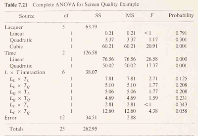
Orthogonal Polynomials (Complete ANOVA)
Book <Fundamental concepts in the design of experiments, C. Hicks 1982>
Page 156,
shows the following figure.
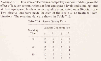
Raw data are
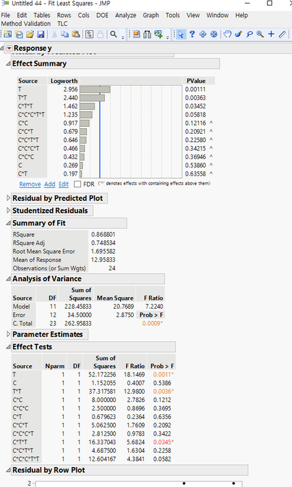
I had tried to create the SAME results as above in JMP, failed.
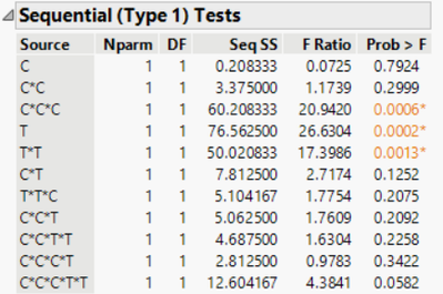
JMP's result is surely wrong since Sum of the SS does not equal to the Model SS. (they should be same.)
So here is my question.
To create the exact same results as the Book, how would I run the JMP??
In above, both C and T were designated as Continuous.
Please inform me. thanks.
Accepted Solutions
- Mark as New
- Bookmark
- Subscribe
- Mute
- Subscribe to RSS Feed
- Get Direct Link
- Report Inappropriate Content
Re: Orthogonal Polynomials (Complete ANOVA) in JMP
Although the results do not match, JMP is not wrong.
Textbooks will often present results that you can match with by-hand calculations. In this case, the results in the book are using what are called Type I Sums of Squares. These sums of squares are additive and easy to calculate by hand. However, the model results will depend on the order that the terms are listed in the model. What this means is that the model Y=intercept + B1*C + B2*T + B12*C*T will be different than the model Y=intercept + B2*T + B1*C + B12*C*T. Since the order that you specify your model can provide different results, Type I Sums of Squares are not often used. This is the root of your issue. Your JMP model was not specified in the same order as the book model. But there is more.
By default, JMP uses what are called Type III Sums of Squares. Type III Sums of Squares calculate the sums of squares for each model term as if it were the last term entered into the model. That means that you will get the same sums of squares and statistical test results regardless of the order that you enter the terms. But, this also means that the sums of squares will no longer be additive. This is why your JMP results do not add up as you would have expected.
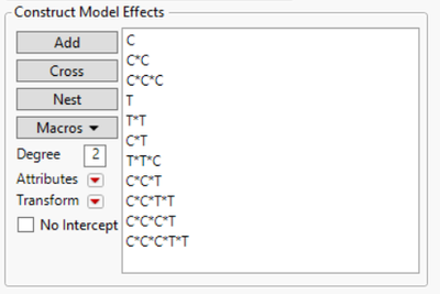
So how do you get your results to match? First, specify the same model order as the book. That means your Fit Model dialog should look like this:
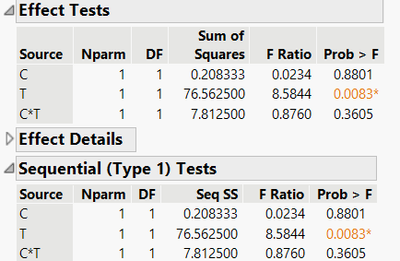
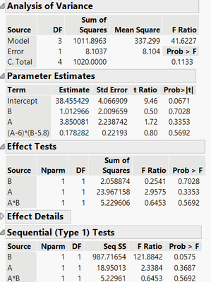
When you run this model, the sums of squares still will not match. However, if you go to the red triangle at the top of the model results and select Estimates > Sequential Tests you will get this report:
These results match the book results.
- Mark as New
- Bookmark
- Subscribe
- Mute
- Subscribe to RSS Feed
- Get Direct Link
- Report Inappropriate Content
Re: Orthogonal Polynomials (Complete ANOVA) in JMP
Now I fully got what was going on.
Thank you so much your answer is deep into the knowledge.
I have few knows about Type 1~3 . sothat this time, I just get as 'OK, there are some ways to get the SS varied.'
However, so, if Type1 result and Type3 result are not consistent, (obviously huge gap in SS)
is it to be more believed on Type3 since that is more prevalent? (jmp rather than books?)
Sincerely. Mike
- Mark as New
- Bookmark
- Subscribe
- Mute
- Subscribe to RSS Feed
- Get Direct Link
- Report Inappropriate Content
Re: Orthogonal Polynomials (Complete ANOVA) in JMP
additionally, I, including many people, are so used to use type I SS, from every text books...
I searched info about type I and III and still cannot abandon the way I am used to.,..
- Mark as New
- Bookmark
- Subscribe
- Mute
- Subscribe to RSS Feed
- Get Direct Link
- Report Inappropriate Content
Re: Orthogonal Polynomials (Complete ANOVA) in JMP
This is not an issue about which is to be more believed. They are just different ways of thinking about the problem. If you have factors A, B, and C, are you okay with the model Y=A+B+C being different than Y=C+A+B? then Type I Sums of Squares are just fine. In some cases Type I makes sense -- think of model hierarchy. Y=A+A^2+A^3 would be a good example where Type I might make sense. Remember that Type III SS would just have each effect listed last in the model order. So, Y=A+B+C would give you the C sums of squares. Y=A+C+B would give you the B sums of squares, and Y=C+B+A would give you the A sums of squares. So the actual mathematics are not really different. Type III is just telling you how much variance that factor explains given that all other terms are in the model. Another way of wording it: once all other factors are considered, how much additional variance does this factor explain? The Type I SS are telling you how much variance that factor explains given the preceding terms in the model (but not the remaining model terms).
Now, not to confuse the issue, but it is important to note that if you truly have orthogonal terms in your model then Type I SS will equal Type III SS, so the difference doesn't matter. You can see this with your example data. Just fit a model of Y=C+T+C*T.
You saw differences in your initial analysis because the quadratic and cubic terms are NOT orthogonal to the other terms in the model. That is the situation where the Type I and Type III sums of squares will not match.
Introductory texts do not want to confuse the issue on the different types of sums of squares because they are introductory. To avoid the issue they will typically use balanced data with orthogonal model terms so the sums of squares would match. This particular example is somewhat surprising because they have balanced data, but added the non-orthogonal quadratic and cubic terms.
- Mark as New
- Bookmark
- Subscribe
- Mute
- Subscribe to RSS Feed
- Get Direct Link
- Report Inappropriate Content
Re: Orthogonal Polynomials (Complete ANOVA) in JMP
I should also add that we have discussed Type I and Type III sums of squares. There is also Type II and Type IV sums of squares (for some reason roman numerals are always used). They are not relevant here, but since you are doing some research, I thought I should mention that there are other ways to calculate sums of squares.
- Mark as New
- Bookmark
- Subscribe
- Mute
- Subscribe to RSS Feed
- Get Direct Link
- Report Inappropriate Content
Re: Orthogonal Polynomials (Complete ANOVA) in JMP
Thank you so much for detailed explanation.
I understand what are your points.
I have curiousity that in what situation Y=A+B and Y=B+A are actually different?
Since we all had been taught that plus-sign-connected terms are 'interchangeable / exchangeable'.
Is there some other meaning of the sequence of the terms for statistical sense?
and One more thing.
I read the type I is not suitable for Factorial Design. (2th page of)
https://www.utstat.utoronto.ca/reid/sta442f/2009/typeSS.pdf
Aren't about all design we use the Factorial Design? little embarassed..
Please let me know what I am wrongly understand..
- Mark as New
- Bookmark
- Subscribe
- Mute
- Subscribe to RSS Feed
- Get Direct Link
- Report Inappropriate Content
Re: Orthogonal Polynomials (Complete ANOVA) in JMP
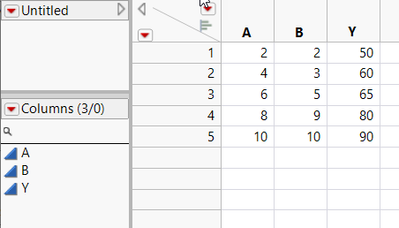
I should be more precise on my wording. You asked what situations have Y=A+B is not the same as Y=B+A. Remember, we are talking about sums of squares which leads to the statistical testing. So your book example already shows this situation. However, here is a simpler example that I just made.
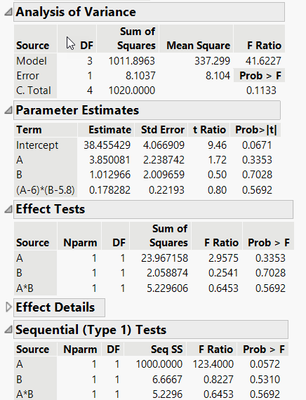
I fit the model Y=A+B+A*B and Y=B+A+A*B. Here are the results for Y=A+B+A*B:
and Y=B+A+A*B
Although the parameter estimates are the same, the statistical testing results are NOT the same when using the Type 1 SS.
Also, remember that statistical models are ESTIMATING the parameter estimates. They are NOT known exact quantities. There is uncertainty in the parameters. But this issue of the statistical testing being order dependent is why Type I Sums of Squares are not often used. People dislike the fact that the order of the model terms can lead to different statistical conclusions and different interpretations of what we think the correct model is. It sounds like you are starting to see why the default in JMP is to use the Type III sums of squares because the order of the model does not matter then.
Finally, factorial designs are only one type of design. There are response surface designs like central composite designs or box-behnken designs. There are fractional factorial designs, There are Plackett-Burman designs. There are optimal designs which have different types such as D, I, A, and G. There are space-filling designs. And so on. So although most people learn about factorial designs first, it is not the only type and I would guess that it is likely not the most commonly used design since there are so many other choices.
- Mark as New
- Bookmark
- Subscribe
- Mute
- Subscribe to RSS Feed
- Get Direct Link
- Report Inappropriate Content
Re: Orthogonal Polynomials (Complete ANOVA) in JMP
Well, what I was asking is, for your example,
When we have two different analysis results,
1) Y=A+B+AB, 2) Y=B+A+BA,
If one changes method 1) to 2), what practical explanation would have changed ?
Is only the user's priority has been changed, like, 'I suppose factor B is more matter so let my equation be 2), then analysis as latter is correct' ?
And my background is like self-study on statistics sothat I always have thought like
1. fractional factorial design < is one special case of the Factorial design
2. CCD < is Factorial design which has additional Center point and consideration of the Orthogonality, whatever else makes analysis more precise.
3. and so on.
It was like, as long as there are 'factors' of interest, I have thought they are all Factorial design..
And this is the off the subject question but I am sure you know.
If 3^3 factorial design was conducted with no replication, (27 measurements)
Done as Complete Randomized Design.
ABC interaction can be partitioned to, 4 parts (each of 2 df),
ABC
ABCC (=ABC^2)
ABBC
ABBCC
(now I found that above terms can be calculated through JMP with inputting Factors like a*b*c*c and a*a*b*b*c which sum up to the ABCC)
normaly, I would have choose ABC term in anova as Error term (supposing several assumptions are met) and go to F test.
However, recently I had noticed that this ABC interaction term can be devided as above,
Thus, if, needed assumptions are met, I can arbitrarily choose whichever of the 4 components to become a Error term?
Like, below 3 cases are all making sense.
case 1) I choose ABCC as Error term (2df)
case 2) I choose ABC and ABCC as Error term (4df).
case 3 ) I choose All the terms as Error (8df)
(of course I know I cannot suggest the practical meaning of choosing this)
Recommended Articles
- © 2026 JMP Statistical Discovery LLC. All Rights Reserved.
- Terms of Use
- Privacy Statement
- Contact Us
