- New to JMP? Let the Data Analysis Director guide you through selecting an analysis task, an analysis goal, and a data type. Available now in the JMP Marketplace!
- See how to install JMP Marketplace extensions to customize and enhance JMP.
- Subscribe to RSS Feed
- Mark Topic as New
- Mark Topic as Read
- Float this Topic for Current User
- Bookmark
- Subscribe
- Mute
- Printer Friendly Page
Discussions
Solve problems, and share tips and tricks with other JMP users.- JMP User Community
- :
- Discussions
- :
- Re: How to get the UCL value for Outlier analysis in a script?
- Mark as New
- Bookmark
- Subscribe
- Mute
- Subscribe to RSS Feed
- Get Direct Link
- Report Inappropriate Content
How to get the UCL value for Outlier analysis in a script?
Hi,
I like to write a script to get the UCL for multivariate outlier analysis using Mahalanobis Distance.
I can get the UCL by going through the JMP menu but is there anyway one can get UCL and set it to variable name in a script.
I appreciate your hlep. Thanks.
Accepted Solutions
- Mark as New
- Bookmark
- Subscribe
- Mute
- Subscribe to RSS Feed
- Get Direct Link
- Report Inappropriate Content
Re: How to get the UCL value for Outlier analysis in a script?
Hi @AT,
It seems a little tricky to lift this value from the report, but you could get at it by scripting the "Save Outlier Distances" action and then pulling out the column property "Mahal. Value" that results from that action. It's not too difficult to get column property values saved as variables. Here's an example using the Thickness sample data set:
dt = Open("$SAMPLE_DATA/Quality Control/Thickness.jmp");
multi = dt << Multivariate(
	Y(
		:Thickness 01,
		:Thickness 02,
		:Thickness 03,
		:Thickness 04,
		:Thickness 05,
		:Thickness 06,
		:Thickness 07,
		:Thickness 08,
		:Thickness 09,
		:Thickness 10,
		:Thickness 11,
		:Thickness 12
	),
	Estimation Method( "Row-wise" )
);

multi << Mahalanobis Distances( 1 , Save Outlier Distances);

mahal_ucl = Column("Mahal. Distances") << Get Property("Mahal. Value");
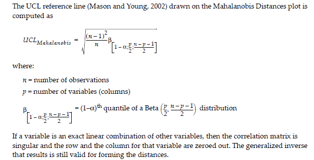
However, this limit is actually really easy to compute in a function. It's just the square root of the the UCL in a Hotelling's T^2 Chart.
Mahal_UCL = function({p,m},
	sqrt(((m-1)^2)/m*beta quantile(0.95,p/2,(m-p-1)/2));
);
The formula is also given in the Multivariate Methods book on page 49 in the Help menu (Help > Books > Multivariate Methods).
Here's an example using the Thickness data. The Mahalanobis control limit is 4.36. Using the previously provided function, you can calculate the Mahalanobis distance UCL for m=50 data points and p=12 variables. Here's the log output showing a matching control limit:
Mahal_UCL(12,50);
/*:

4.36283881449635
The function Mahal_UCL I wrote hard-codes in alpha = 0.05. You could make alpha a 3rd parameter like so:
Mahal_UCL = function({p, m, alpha},
	sqrt( ( ( m-1 )^2 )/m*beta quantile( 1-alpha, p/2, ( m-p-1 )/2 ) );
);
- Mark as New
- Bookmark
- Subscribe
- Mute
- Subscribe to RSS Feed
- Get Direct Link
- Report Inappropriate Content
Re: How to get the UCL value for Outlier analysis in a script?
Thanks so much for your help Cameron. This is very helpful.
- Mark as New
- Bookmark
- Subscribe
- Mute
- Subscribe to RSS Feed
- Get Direct Link
- Report Inappropriate Content
Re: How to get the UCL value for Outlier analysis in a script?
Hi @AT,
It seems a little tricky to lift this value from the report, but you could get at it by scripting the "Save Outlier Distances" action and then pulling out the column property "Mahal. Value" that results from that action. It's not too difficult to get column property values saved as variables. Here's an example using the Thickness sample data set:
dt = Open("$SAMPLE_DATA/Quality Control/Thickness.jmp");
multi = dt << Multivariate(
	Y(
		:Thickness 01,
		:Thickness 02,
		:Thickness 03,
		:Thickness 04,
		:Thickness 05,
		:Thickness 06,
		:Thickness 07,
		:Thickness 08,
		:Thickness 09,
		:Thickness 10,
		:Thickness 11,
		:Thickness 12
	),
	Estimation Method( "Row-wise" )
);

multi << Mahalanobis Distances( 1 , Save Outlier Distances);

mahal_ucl = Column("Mahal. Distances") << Get Property("Mahal. Value");
However, this limit is actually really easy to compute in a function. It's just the square root of the the UCL in a Hotelling's T^2 Chart.
Mahal_UCL = function({p,m},
	sqrt(((m-1)^2)/m*beta quantile(0.95,p/2,(m-p-1)/2));
);
The formula is also given in the Multivariate Methods book on page 49 in the Help menu (Help > Books > Multivariate Methods).
Here's an example using the Thickness data. The Mahalanobis control limit is 4.36. Using the previously provided function, you can calculate the Mahalanobis distance UCL for m=50 data points and p=12 variables. Here's the log output showing a matching control limit:
Mahal_UCL(12,50);
/*:

4.36283881449635
The function Mahal_UCL I wrote hard-codes in alpha = 0.05. You could make alpha a 3rd parameter like so:
Mahal_UCL = function({p, m, alpha},
	sqrt( ( ( m-1 )^2 )/m*beta quantile( 1-alpha, p/2, ( m-p-1 )/2 ) );
);
- Mark as New
- Bookmark
- Subscribe
- Mute
- Subscribe to RSS Feed
- Get Direct Link
- Report Inappropriate Content
Re: How to get the UCL value for Outlier analysis in a script?
Thanks so much for your help Cameron. This is very helpful.
Recommended Articles
- © 2026 JMP Statistical Discovery LLC. All Rights Reserved.
- Terms of Use
- Privacy Statement
- Contact Us

