- Subscribe to RSS Feed
- Mark Topic as New
- Mark Topic as Read
- Float this Topic for Current User
- Bookmark
- Subscribe
- Mute
- Printer Friendly Page
Discussions
Solve problems, and share tips and tricks with other JMP users.- JMP User Community
- :
- Discussions
- :
- Re: Graph for Response Surface Methodology

- Mark as New
- Bookmark
- Subscribe
- Mute
- Subscribe to RSS Feed
- Get Direct Link
- Report Inappropriate Content
Graph for Response Surface Methodology
Hi, JMP experts, this question has been bothering me for a long while. I hope to get answered with your help.
I am trying to do RSM with one DV and two IV, all continuous and I am wondering how to create a three dimensional graph as shown in attached. I saw that graph in a paper that uses similar designs, and hope that JMP has this function of creating this graph. Thank you!

Accepted Solutions

- Mark as New
- Bookmark
- Subscribe
- Mute
- Subscribe to RSS Feed
- Get Direct Link
- Report Inappropriate Content
Re: Graph for Response Surface Methodology
I assume that you used JMP to design the experiment and store the design in a JMP data table. Furthermore, I assume that you fit the RSM model using Analyze > Fit Model or by running the Model table script.
At this point you want to use a profiler. Click the red triangle next to Fit Least Squares and select Factor Profiling > Surface Profiler. You can read about this profiler in Help > Books > Fitting Linear Models.
- Mark as New
- Bookmark
- Subscribe
- Mute
- Subscribe to RSS Feed
- Get Direct Link
- Report Inappropriate Content
Re: Graph for Response Surface Methodology
I should add that the reason for the omission of the use of color as you see in the MINITAB example is not an oversight. JMP uses color in the Contour Profiler to indicate regions of disallowed response values. You can set the low or high limit and see what I mean. The color is determined by the response. If you have multiple responses, they can all be viewed simultaneously with their individual disallowed regions as transparent, overlaid shaded areas. The white are is the region where the response will satisfy all of the limits.
- Mark as New
- Bookmark
- Subscribe
- Mute
- Subscribe to RSS Feed
- Get Direct Link
- Report Inappropriate Content
Re: Graph for Response Surface Methodology
I assume that you used JMP to design the experiment and store the design in a JMP data table. Furthermore, I assume that you fit the RSM model using Analyze > Fit Model or by running the Model table script.
At this point you want to use a profiler. Click the red triangle next to Fit Least Squares and select Factor Profiling > Surface Profiler. You can read about this profiler in Help > Books > Fitting Linear Models.
- Mark as New
- Bookmark
- Subscribe
- Mute
- Subscribe to RSS Feed
- Get Direct Link
- Report Inappropriate Content
Re: Graph for Response Surface Methodology
Hi, Mark thank you so much. So helpful!
A follow-up question: is there a way to produce a contour plot as show in attached picture? I saw this plot in a study with RSM done in Minitab. Thank you a million!

- Mark as New
- Bookmark
- Subscribe
- Mute
- Subscribe to RSS Feed
- Get Direct Link
- Report Inappropriate Content
Re: Graph for Response Surface Methodology
Follow the instructions above but select the Contour Profiler. Be sure to read the chapter about this profiler in the same guide book! Especially the part about the Contour Grid command.
Additionally, select Graph > Contour Plot. This platform is documented in the Help > Books > Essential Graphing guide book.
There is a lot of support for contour plots but you have to read up a bit to find the commands and options that produce the result that you want.
- Mark as New
- Bookmark
- Subscribe
- Mute
- Subscribe to RSS Feed
- Get Direct Link
- Report Inappropriate Content
Re: Graph for Response Surface Methodology
Hi, I just checked out the resources you pointed to, and came up with the attached graph from the Fit Model-RSM. It is starting to look like the one from the published paper, but not quite. Is there a way to fill in the color as in the paper? Am I missing something? Thank you!

- Mark as New
- Bookmark
- Subscribe
- Mute
- Subscribe to RSS Feed
- Get Direct Link
- Report Inappropriate Content
Re: Graph for Response Surface Methodology
Data is attached here in case you want to play with it. Thank you!
- Mark as New
- Bookmark
- Subscribe
- Mute
- Subscribe to RSS Feed
- Get Direct Link
- Report Inappropriate Content
Re: Graph for Response Surface Methodology
It is not possible to fill in the isometric areas with color in the Contour Profiler as far as I know.
You can produce colored regions in the Contour Plot if you save the model as a column prediction formula.

Select the Fill Areas command from the red triangle. You can change the color by selecting the Color Theme command in the same menu.
- Mark as New
- Bookmark
- Subscribe
- Mute
- Subscribe to RSS Feed
- Get Direct Link
- Report Inappropriate Content
Re: Graph for Response Surface Methodology
I should add that the reason for the omission of the use of color as you see in the MINITAB example is not an oversight. JMP uses color in the Contour Profiler to indicate regions of disallowed response values. You can set the low or high limit and see what I mean. The color is determined by the response. If you have multiple responses, they can all be viewed simultaneously with their individual disallowed regions as transparent, overlaid shaded areas. The white are is the region where the response will satisfy all of the limits.
- Mark as New
- Bookmark
- Subscribe
- Mute
- Subscribe to RSS Feed
- Get Direct Link
- Report Inappropriate Content
Re: Graph for Response Surface Methodology
Thank you Mark. Your answer is very helpful, as always.
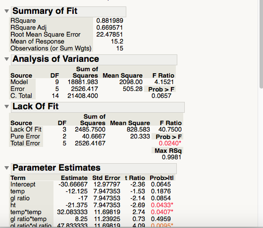
One more question about RSM. In Sample Data Library, the Oder Control Original Dataset was used to demonstrate RSM. I saw that the in the Analysis of Variance section, F=4.15, and p=0.06, which means the model is not significant at alpha=0.5. In multiple regression, I have been taught that you donot go on when your overall model is not significant. Does the same rule apply in RSM models? Do you have reference on this aspect? Thank you!
- Mark as New
- Bookmark
- Subscribe
- Mute
- Subscribe to RSS Feed
- Get Direct Link
- Report Inappropriate Content
Re: Graph for Response Surface Methodology
We use objective methods (e.g, design of experiments, analysis of variance, linear regression) that involve subjective decisions. What level of alpha should I use for my inference? Do I also consider the importance of a factor as well as its statistical significance? Also, there are many statistics and criteria available besides the F ratio that is testing the significance of the whole model. Which ones should I use? How do they work and how do they inform me?
So a p-value of 0.0657 for a F ratio of 4.1521 with only 5 degrees in the denominator is not an especially a strong hypothesis test. 9 DF were given up to fit the whole model. If I eliminate unimportant and insignificant terms (ht*temp, ht*gl ratio, ht*ht, and gl*temp), the F ratio is 11.2338 with 9 DF in the denominator, almost twice as many and the p-value is now 0.0012. The R square and adjusted R square a more in line with each after reducing the model. The first model was over-fitting and that, among other things, weakened the test.
It is the age of 'big data' but we must still strive to use all the methods developed for small data sets such as this example with careful consideration. There is no Easy button to be had.
Recommended Articles
- © 2026 JMP Statistical Discovery LLC. All Rights Reserved.
- Terms of Use
- Privacy Statement
- Contact Us