An Agile Cause Analysis Using JMP ®

3 Kudos

Cause Analysis

Georgia Z. Morgan, Sr Statistician, Retired

Cause analysis is a general term applied to the tasks used to investigate, analyze and eventually determine the causal factors of a single, or multiple, anomalies. Advanced machine learning methods and other data mining tools have reduced the time and effort to analyze data.

Data prep, the steps to acquire data and transform it into information, require domain expertise. To root cause a complex, manufacturing process, it is likely that the domain experts are from different functional organizations and the data from different sources.

My experience is shared by others:

“Often, the data is in different systems and needs to be accessed and turned into a data set that can be used for data mining and machine learning. …

This often requires a significant amount of data aggregation and transformation. Once a single analytics base table for the analysis has been aggregated, the other aspects of the life cycle come into play. Because it is necessary to experiment with data, the preparation stage is also very iterative with the analyst trying different types of data to get the most accurate predictive results.”

(n.a.), (n.d.), Data Mining from A to Z. Retrieved July 31, 217 from the SAS website https://www.sas.com/content/dam/SAS/en_us/doc/whitepaper1/data-mining-from-a-z-104937.pdf

“As I’ve noted on countless occasions, there is a tremendous difference between mining data and answering questions. Any given dataset offers a particular glimpse onto reality, but no single dataset offers a perfect, holistic and unbiased view of the entirety of all existence. This means that when it comes to analyzing data, in many ways it is far more important to have any understanding of the data one is looking at than it is to have a PhD in statistics.”

Leetaru, K. (June 12, 2016) Why We Need More Domain Experts In The Data Sciences. Retrieved July 31, 2017 from the Forbes website https://www.forbes.com/sites/kalevleetaru/2016/06/12/why-we-need-more-domain-experts-in-the-data-sci...

It is also my experience that:

Most data iterations are time consuming.
Joins are almost always offline, so each iteration requires another meeting, in other words,
Not agile!

This presentation has two goals. My primary goal is to demonstrate how the JMP Virtual Join can help a root cause analysis team be more agile, when it comes to combining tables. My secondary goal is to gather alternate proposals for the cause analyses that will be presented. The example is hypothetical in that it does not describe an actual problem that I have seen, but is based upon several experiences of what can go wrong. Also, all of the data is simulated. While this example will draw from semiconductor (IC) manufacturing, this problem could happen to any processing factory or even in drug studies.

A brief overview of aspects of IC manufacturing, to provide context for the data and anomaly, will be followed by some details about Virtual Joins, and then the analyses. Note, the example presented here is one of two that are written up in the attached paper.

Keywords: anomaly, RCA (Root Cause Analysis), data mining tools, semiconductor manufacturing, JMP® virtual join, JSL, reentrant process, IC (integrated circuit), FEOL (Front End Of Line), BEOL (Back End Of Line), EOL (End Of Line, typically, yield and performance testing and Die Prep), PM (Preventive Maintenance).

Some Context

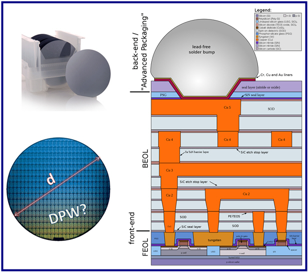
Integrated Circuits, ICs, are created from numerous processing steps of: oxidation, implantation, deposition of films and sputtered metals with different conductivity and barrier (non-conductivity) characteristics, patterning, planarization, and of course cleaning and measurement. It starts with a bare, doped silicon wafer [1] and ends up with multiple die (ICs) per wafer. The maximum number of die per wafer depends upon the wafer size (diameter) and die size[2]. See Figure 1(L)

Figure 1(R) is a cartoon depicting a very small segment of a chip with a 5-layer Cu metal interconnect BEOL.[3] Even though the architecture, metal thickness, layout and possibly the recipe, might be different for each Cu layer, typically, they are processed in the same factory area (fab bay) and on the same tools.

Figure 1 (L) Carrier of 25 bare silicon wafers with flat and fully processed wafer with notch (R) An IC graphic of a five layer Cu interconnect BEOL.

The FEOL and BEOL are segmented. Even a minute amount of Cu quickly diffuses through oxides creating defects and degrading the gate oxide quality.

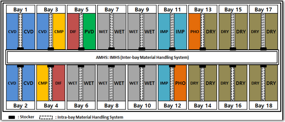
Figure 2 depicts a possible fab (factory) layout for a FEOL [4]. Processing equipment of the same type and function are located in bays. Their layout is optimized for plumbing to bulk chemical delivery, exhausts and drains. An overhead rail system, called an automatic material handling system (AMHS) carries fab lots from one station to the next, or temporarily stores them in a remote stocker until a tool becomes available. There is no standard layout, each semiconductor corporation has its own factory planning group. Most of the factory queues are reentrant. For example, the four tools in Bays 7 and 9 might perform seven different clean steps. Knowledge of the factory flow and equipment usage is essential for root cause analysis. Using this example, a single tool could potentially affect a fab lot up to seven times, and some fab lots might never have been processed on that piece of equipment.

See the references [7] or do a quick web search for videos and other sources to learn more about semiconductor manufacturing.

Figure 2 Possible fab layout for a FEOL process.

Processing sequences, time between steps, when it was processed on a specific tool and handling can be important contributing factors to an anomaly, a problem that affects the IC quality. Each silicon wafer has a wafer number scribed into the silicon. There is an industry standard that can trace each wafer to its origin. For about 20 years, fab (factory) processing equipment and handlers have RFID readers. Manufacturing systems capture the exact time wafers enter and exit a tool and more. The simulation data presented (and attached) uses a simple numbering system. It is not a replica of fab data, but provides the desired characteristics for this example.

Virtual Join

A Virtual Join:

Allows a main table to link to multiple auxiliary tables without physically joining them.
Requires two column properties to be set: Link Reference (main table) and Link ID(auxiliary table).
Columns of the referenced (linked) data table are displayed as grouped variables in the main table.
These columns can be used in formulas, graphs, analyses and table commands.
Can be created from the UI and can be created and managed using JSL.

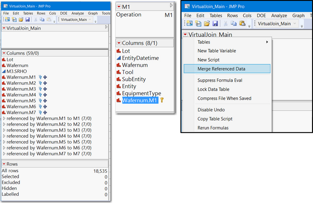
Figure 3 (L) depicts 7 joined tables, they are joined by the unique wafer number (Wafernum). The Link Reference is displayed as a blue shadowed key when linked and gray when unlinked. Click on the disclosure icon to reference the columns for that table.

Figure 3 (L) EOL Yield/Performance/Anomaly Data Virtually Joined with Equipment Data for 7 Operations, (M) M1 Auxiliary Table Panel with Link ID, (R) Table Menu, Merge Referenced Data,

Figure 3 (M)Depicts the table panel for one of these tables (M1, the first Cu layer). The Link ID is a gold key. The Link Reference and Link ID must be the same data type. The Link ID values must be unique, no duplicate values. If using JSL, or to be able to re-link tables in another session, the tables need to be saved to the disk. The list below provides some characteristics of virtual joins. Figure 3(R) shows that at any time a selected set of table links can be merged. Select the Link References to be merged, or select none for all linked columns, then select Merge from the main table menu. It is as easy as that to merge them into the main table.

Items to Note

The path is case sensitive, but a pathname is not required, if the auxiliary jmp data table is in the same directory as the main data table. (Use posix syntax c:/temp/ if team works with a mix of different operation systems).

For fab data, typical links would be Lot, Wafer ID, maybe Die (row, column). The RCA team should agree on a standard, and each area representative should own their data, and prepare by creating the Link ID. This allows for data corrections in parallel with RCA meetings and can be easily linked once ready.

Don't use a DB name for the links, since each linked table requires a unique Link Reference and corresponding Link ID. Use a function for the links. Updating data will be easier and the Link value is updated as well. ( Each Wafernum.M<x> column uses a column formula for the DB column Wafernum.)

Saved platform scripts use a verbose syntax to reference a linked column.
Referenced Column( "Tool[Wafernum.M1]",
Reference( Column(:Wafernum.M1), Reference(Column( :Tool ))))

This simpler syntax seems to work.

:Name("Tool[Wafernum.M1]") in other words, :Name("colname[Link ID]")

Close the auxiliary table, rather than unlinking, especially, if the link might be used later, possibly for a different file.

Recommended:

Create an add-in or scripts to automatically create links, and open established link files.

Virtual Join Benefits:

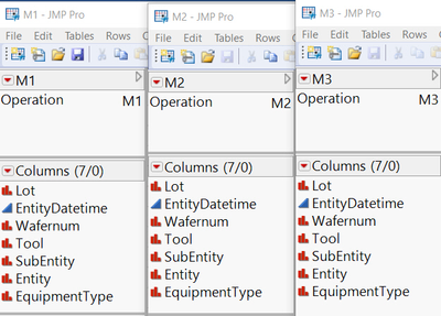
Column name management Figure 4 shows 3 of the 7 linked tables. They each have the same column names. All JMP joins adds information about the source table for columns with the same names, however, the names are the source table names which are often long and complex. For a Virtual Join, you set the Link Reference and Link ID names. With the less verbose syntax, name management is easier and more readable for linking, and scripting.

Working in parallel Suppose the cause analysis team member for M5 stated that his data had a problem. Close the M5 data table, let the team continue and when ready, open the corrected table and relink it with a right click on the main table column Wafernum.M5 and select Link Reference. A list of files appear and select the M5 file.

Figure 4 Fab Equipment Data for 3 Operations, Same Column Names

Simulated Example - Intermittent Failing EOL M3 Resistance

One of the more difficult causes to root out is a contamination problem, especially if the contamination is removed with scheduled maintenance (PM) and dissipates with usage (repairable) and if it is conditional. A simulation of for a BEOL semiconductor manufacturing fab for a 7 layer metal sputter was created to demonstrate this anomaly.

Epidemiology, drug studies and food and drug processing likely experience a similar type of anomaly at some frequency.

SRHO is a metal resistance quality metric. There is no shortage of potential causes for an increase in SRHO, even restricting the investigation to just the M3 loop. If lines are too narrow resistance increases. If lines are cracked or other defects or metal contamination can affect the metal conductive characteristics. Figure 5 displays the effect. The top graph represents baseline material for several weeks before a holiday shutdown. The bottom graph depicts post-holiday material. A few intermittent lots’ EOL indicators for M3 resistance fail SPC, and are so far out of control, wafers must be scrapped. There were only a few anomalous lots, then none were seen. Then the “eventual rule” kicks in: small signals eventually become large signals. A flurry of bad lots appear at the end of line.

Figure 5 M3.SRHO (T) Baseline Lot Avg (B) Post-Holiday Lot Avg versus M3 Sputter Tools

Cause Analysis Questions

Is the anomaly tool specific?
Are the processes consistent, use the same chemicals?
Given the intermittent nature, could this be related to the tool state?
Could this be related to process sequence, queue times, time between one step to another, etc.

Only M1-M7 sputter was simulated with a FIFO queue, with an exception. Full lots are 25 wafers, half lots are 12 wafers, and quick turn lots are 6 wafers. The FIFO exception is that a 6 wafer lot takes precedence. To add some reality to the simulation, random throughput times for "other" process steps were used to have varying reentrant times between M1 and M2, etc. These other processing times were based upon fixed setup times; processing time based upon the number of wafers and precedence; and random queue times. In a real cause analysis with real data, each tool and queue in the loop needs investigation. Only the sputter tools were simulated to limit complexity and focus on methods. Also note, the paper uses the narrative that inline critical dimension data showed no change in line size. To eliminate line breakage or cracks, typically a strip back or inline visuals are reviewed. Nothing was found so the focus is on the metal itself.

To answer question #1, a comparison of incidence by tools is reviewed. Most often this is a one tool at a time review done by the modules and reviewed at the first RCA team meeting. Or a data mining tool with feature selections could be applied to a massive table with columns from multiple steps. Instead of a single monolithic file, a virtually linked main table like the one seen in Figure 3 (L) could be used.

Question #2, to continue the narrative, a chemical review of the bulk systems finds nothing. All tools are plumbed to the same systems. At this point, the anomaly data could be linked with tables of inline monitor data, tool sensor data and analyzed.

As the narrative continues, an engineer states that a couple weeks before shutdown, the M5 recipe, the chemical mix was changed to make the deposition more conformal to the topography (structures) at M5. The characterization prior to implementation included a few M5 wafers followed by a few wafers of M1, and repeated for the other layers. All results were within baseline.

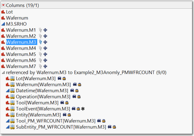
The RCA team chair asks for an analysis of wafer counts for both M3 and M5, trying to answer question #3, about tool state. Suppose the engineer's first file only had total wafer counts. Close the table and have the engineer add a column for the cumulative number of M5 wafers run prior to M3. When the data is modified, open the new file and link. Figure 6 demonstrates tha different files, different iterations can be linked to the anomaly data.

Figure 6 Post-Holiday EOL M3 Anomaly Data Linked with M3 Tool PMCounters

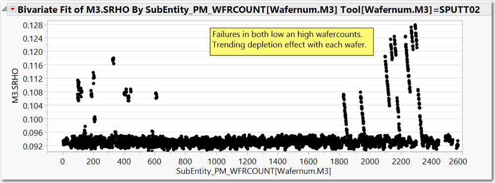
Figure 7 - Post-Holiday M3.SRHO versus PM_WFRCOUNT by Tool (only SPUTT02 shown here)

Figure 7, a Fit Y by X plot of M3.SRHO data versus wafer counts for SPUTT02 demonstrates that failures occurred with low wafer counts and high wafer counts. The simulation scheduled SPC every 500 wafers and a PM is done after 5000 wafers or about 2500 wafers per chamber. There seems to be a depletion effect seen on the full lots (a decrease with each wafer). Also, due to the nature of this simulation, early post-holiday material had many 6 wafer, quick turn lots.

Given that the pre-implementation characterization showed no effect with only a few M5 wafers run, could this be an accumulation or due to sequencing, in other words, question #4?

For past analyses, I have used event analyses for my next steps.

Create a table of all tool events. (MES data for the sputterers.)
Create columns representing 10 or more lags. This is easier to do by tool. The steps are: Subset by tool. Write a script to create lags (see lagit.jsl) Combine the tool files.
Select the M3 operation data, since this potential tool state anomaly only seems to affect M3. That is use only M3 rows. See file M3 Last 20.jmp. Create the Link ID Wafernum.M3.
Open this file and from the anomaly data right click on column Wafernum.M3, select Link Reference . Use tree methods (Partition) and feature selection to find a pattern.

Event sequencing can be done, fairly quickly using the JMP function Lag( :col, n ), which works on character columns. In this case, the tool histrory, what the tool has run previously, is created.

Figure 8 Snippet of table M3 Last 20.jmp Structure with lags of Tool Events

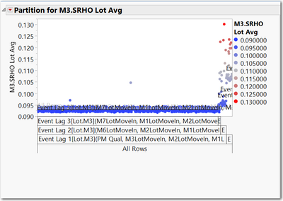
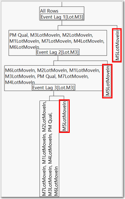
Figure 9 Partition of M3.SRHO Lot Average vs. Last 20 Tool Events

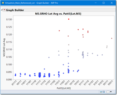
Figure 8 displays a snippet of the table structure and Figure 9 the Partition history. Lags 1, 2 and 3 were chosen in order, and each time, splitting on the event M5LotMoveIn. Figure 8 displays a formula column to simplify the sequencing. It is the concatenation of coded events, 0 = PM, 5=M5 and 1 for all other events. Figure 10 is the graph presented for the RCA management update.

Figure 10 Presentation Graph of M3SRHO Lot Processing Effect

Comments

The simulation achieved the intended affect.
Standard modeling of this type of anomaly is difficult due to built-in saturation, PM and depletion.
Sequencing, and looking for specific effects is (was) my BKM.
- Find all M3 lots where M5 was run just prior.
- Compute the delta to baseline. Compare the effect to the number of wafers.
- Investigate the wafer depletion effects.

Currently, I am researching reliability sequencing and looking for suggestions for standardizing these methods.
The paper contains more details, and another cause analysis example. The attached data folder contains readme.txt files regarding the simulation and the modeled effect. The data files once linked have attached scripts to recreate the graphs and partition.

Virtual Joins make for agile data updates and restructuring, which is especially useful for RCA.

References

[1] Figure 1(L) Bare Silicon Wafer, (n.a.), (n.d.), Silicon Wafer. Retrieved July 31, 2017, from TechInstro website, https://www.techinstro.com/silicon-wafer/

[2] Figure 1 (L) , (n.a.), April 09, 2013, Die Per Wafer Formula and (free) Calculator. Retrieved July 31, 2017, from anysilicon website, http://anysilicon.com/die-per-wafer-formula-free-calculators/

[3] Figure 1(R) (n.a.), (n.d.), Back End of Line. Retrieved July 31, 2017 from Wikipedia, The Free Encyclopedia, website, https://en.wikipedia.org/wiki/Back_end_of_line

[4] Figure 2, 유광재, January 20, 2015, Optimal Fab SDM LAB, KAIST Industrial & Systems Engineering, Figure 2. Optimal FAB layout design based on the material flow among the process types. Retrieved July 31, 2017, from http://sdm.kaist.ac.kr/wordpress/korean/%EC%9C%A0%EA%B4%91%EC%9E%AC/, http://sdm.k aist.ac.kr/wordpress/korean/wp-content/uploads/sites/2/2015/01/YGJ_2.png.

[5] Leetaru, K. (June 12, 2016) Why We Need More Domain Experts In The Data Sciences. Retrieved July 31, 2017 from the Forbes website https://www.forbes.com/sites/kalevleetaru/2016/06/12/why-we-need-more-domain-experts-in-the-data-sci...

[6] (n.a.), (n.d.), Data Mining from A to Z. Retrieved July 31, 217 from the SAS website https://www.sas.com/content/dam/SAS/en_us/doc/whitepaper1/data-mining-from-a-z-104937.pdf

[7] Other websites to learn more about semiconductor manufacturing

https://www.bloomberg.com/news/articles/2016-06-09/how-intel-makes-a-chip

https://www.youtube.com/watch?v=vmAyXWvLHeI (FOUP Load Movie)

https://www.youtube.com/watch?v=4Q_n4vdyZzc (Semiconductor Technology at TSMC, 2011)