Speeding Up the Dirty Work of Analytics

2 Kudos

SPEEDING UP THE DIRTY WORK OF ANALYTICS

Robert H. Carver rcarver , Professor of Business Administration Stonehill College, Easton MA 02357, (508-565-1130), rcarver@stonehill.edu and Senior Lecturer, Brandeis University International Business School, rcarver@brandeis.edu

(view in My Videos)

Abstract

“Big data” is rarely ready for analysis when it arrives on your desktop. The issues are familiar, yet they aren’t often what comes to mind in discussions of the “Sexiest Job of the 21st Century.” These are tasks that consume a massive fraction of project time, yet receive comparably little attention in textbooks, professional journals or blogs. The dirty work includes activities such as assembling a data set from disparate sources, exploring data for various forms of messiness, imputing and otherwise addressing missing data, identifying and dealing with outliers, recoding observations to regularize inconsistencies and reduce dimensionality. Fortunately for JMP users, the latest versions of JMP provide intuitive and highly visual tools to perform diagnostics and automate some of the nastier janitorial chores in the analytics workflow. This presentation demonstrates some of the ways that the Query Builder, other Tables menu platforms and Column utilities can expedite the dirty work with some large, publicly available data sources.

Introduction

Although reliable estimates are hard to come by, there seems to be consensus that data preparation – locating, assembling, reconciling, merging, cleaning, and so on – consumes something like 80% of the time required for a statistical project. It’s clear that successful analyses emerge from a disciplined process similar to the one shown here, it is also clear that the process stages (a) proceed iteratively and (b) are rarely depicted with an accurate time scale.

Figure 1: SAS Analytics Life Cycle

The “Prepare” stage is often considered the “dirty work” or janitorial work of analytics. While dirty work may be an apt phrase, it is decidedly negative and underplays the creative, varied, and substantive aspects of the associated tasks.

Inspired by the recent Rio Summer Olympics, in this talk I suggest that the data preparation phase of an analytics project is akin to a blend of Olympic events: imagine a triathlon with obstacles. Each project has hurdles that are predictable yet unique to the process. As a context for the talk, we consider the early stages of a project to investigate the question, “What accounts for differences in Olympic success across nations?” Along the way, we will use some JMP functionality that can considerably speed the phases of data preparation, focusing in particular on some newer commands and platforms.

Danyel Reiche has studied the question of national performance in the Olympis, and wrote in The Washington Post that size, wealth, and policy are key factors– “In “Success and Failure of Countries at the Olympic Games,” I propose the “WISE” formula that helps explain Olympic success. WISE stands for promoting women in sports; institutionalizing national sports promotion; specializing in particularly promising sports; and early adoption of such trends as newly added disciplines.” (Reiche, 2016)

To illustrate the basic approach, we’ll compile a data table relevant part of Reiche’s formulation. In particular, we’ll combine historical medalist data with variables related to national size, wealth, health, and gender equity. Because the focus here is on data preparation, we’ll stop well short of model-building and instead focus on the distinctly “unglamorous” steps required between the Ask and Explore steps of the process. The paper describes the process, providing detailed instructions related to the newer features of JMP and simply describing some of the more familiar and standard phases. Readers should note throughout the extent to which JMP’s features facilitate the workflow and document the process via automatic script generation. Though we won’t engage in any script-writing per se, the value of the built-in scripting is crucial for reproducible research.

Obtaining data

Before gathering the data, there were some decisions to make based on both the logic of the study and the availability of data. Prior studies have tended to look at a small number of prior Olympic editions and at either Summer or Winter games. Here we will look at Summer games between 1960 and 2008 largely due to data availability and the desire to have at least one edition as a holdout sample. We’ll also investigate just those countries that participate in the games currently, noting that this involves some compromise because over the period since 1960 some country names have changed, some have been born, and other nations have vanished.

Another issue with selecting countries is that the Olympic movement and the World Bank (a great source of economic and demographic data) identify countries with different coding schemes. For example, to the Bank Hungary is HGR, but it is HUN to the International Olympic Committee (IOC). Hence, in addition to locating data about each country we also need a translation table to match country rows.

The data for the project come from four sources:

Olympic Medals database, freely available via Microsoft Azure – all medalists between 1900 and 2008.
World Development Indicators (WDI) from the World Bank (1960 – 2015)
List of all countries participating in the Olympics, from Wikipedia.
Comprehensive country codes table (CCC), from data.okfn.org listing numerous standard coding schemes for countries.

The WDI and CCC were downloaded as *.csv files from their respective websites, and read into JMP tables quite easily simply by opening the files. The table from Wikipedia was accomplished with JMP’s Internet Open platform, described next, and the medals database made use of one of JMP’s database functions.

Internet Open

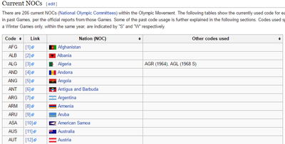
A quick search for a definitive list of IOC countries led me to Wikipedia, specifically to https://en.wikipedia.org/wiki/List_of_IOC_country_codes, with a detail of the result shown in Figure 2. To quickly open the data as a JMP table, we use File > Internet Open… and first specify the URL (see Figure 3). Copy and paste the URL into the dialog as shown, and specify that you want to open is as Data.

Figure 2: IOC Country Codes

12445_fig 2.png

Figure 3: Internet Open

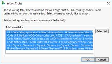
Next comes a dialog (Figure 4) showing JMP’s “best guess” about the presence of tabular data on the particular web page. In this instance, we want the data residing in the second table, so just change the highlighting and click OK.

Figure 4: Selecting Web Page Tables to Import

This immediately opens a new data table, a closeup of which is shown in Figure 5. It consists of four Nominal columns and 206 rows, corresponding to the 206 IOC nations. Also notice that the second column has embedded code referring to the name of the country and the URL for the national flag. Notice further that there are two scripts among the table variables (upper left) titled “Source” and “Load pictures for “Nation (NOC)”. Clicking the green arrow runs the script, and right clicking on the name of the script offers the option to Edit (and thus view) the script. The “Source” script is a record of the Internet Open command that produced the table in the first place; running it again re-opens the table anew, which might be helpful in the future should the country list change in any way. Additionally, once the data table is saved, the script is preserved.

Running the second script adds a new column to the data table (see Figure 6). For later visualizations, it might be handy to have those flag images as an Expression data type in our table.

Figure 5: The Imported Table

Figure 6: National Flags Unfurled

Grabbing a Database Table

As noted earlier, the Microsoft Azure sample databases include Olympic medalist data. There is actually a small database on the server consisting of four tables, but all of the data that we’ll require resides in one table called “Medalist” so the simplest approach here is to connect to the database and import the one table.

Making a Remote Connection

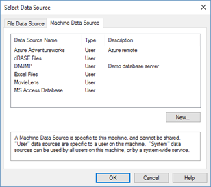
To start, choose File > Database > Open Table. This opens the Database Open Table dialog, which asks you to specify a connection. It is beyond the scope of this presentation to go through the steps of establishing the initial connection to the Azure site; consult your machine settings to make a new ODBC connection if necessary. Having previously entered the specifications we click New Connection (not shown) and the Select Data Source dialog appears. Click on the Machine Data Source tab as in Figure 7. We’ll select the source of interest (Azure Adventureworks) and click OK here.

Figure 7: Selecting a Remote Connection

An authentication dialog will open; after supplying the credentials, click OK.

The Database Open Table dialog (Figure 8) will open again, this time showing the contents of the new remote connection. We’ll proceed now to import the entire table.

Import an Entire Table

We highlight the olympics schema and the table of interest and click Open Table.

Figure 8: Selecting a Table to Open

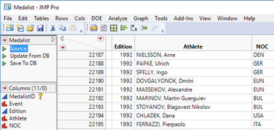
The table will open in a JMP data table window with familiar layout and features, with a few noteworthy elements. As shown in Figure 9, in the left uppermost pane of the window are three green triangles associated with scripts to re-load the table altogether, to update the table from the database or to save revisions to the database. Once we save the data table locally, these scripts allow us to reproduce the import or carry out updates.

The one other noteworthy item here is the identification of the MedalistID column as a key field, or Link ID, witin the database. With a single table, the LinkID property has little impact. If we were to import other tables with a shared Link ID, we could join or perform other database operations.

Figure 9: Data Table Imported from a Database

Import a Subset of a Table

For this study, our interest is in Summer Olympic events from 1960 onward, and that we only want to focus on particular columns for analysis. For very large tables, there might be an efficiency gain from importing only the data we actually expect to use rather than importing the entire table.

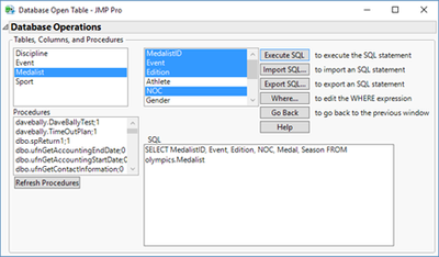
To choose rows and columns for import we want to build a query. The Advanced… button in the Database Open Table dialog (see Figure 8 above) provides a tool (Database Operations subdialog) to construct and execute a query. In this example, illustrated in Figure 10, the default SQL code will select all rows and columns from the particular table.

To choose only some columns, we highlight the columns of interest and they are added into the SELECT statement within the SQL area of the dialog.

Figure 10: Starting to Build SQL Code

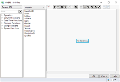
We want Sumer Olympic results starting in 1960, so we need a compound WHERE clause filtering by values of two different columns. To choose a subset of rows, we need to add a WHERE clause. Click the Where… button, opening the dialog shown in Figure 11.

Figure 11: Constructing a WHERE Clause

The Vendor Name Browser (initial value = Generic SQL) is a dropdown list of supported vendor SQL dialects. Choose the one that corresponds to the data source.

The Event column corresponds to year, and we want all years greater than 1960. Click the gray triangle next to Operators to specify the form of the statement. Choose A > = B.

In the list of column names, choose Edition. At this point the formula editor area of the dialog should look like Figure 12. Move the cursor into the empty gray rectangle in the formula editor, double-click, and type 1960, and press Enter.

Figure 12: Building the Formula in the First WHERE Clause

Now we want a second condition, namely to import only rows from Summer Olympic events:

In the formula editor, click anywhere outside of the formula. In the Operators list, click AND to add the second part of the statement.

Select A=B as an operator.

From the list of column names, choose Season.

Finally, move the cursor into the rightmost rectangle, double-click, and type ‘Summer’ within single quotes and click OK, which returns you to the Database Open Table dialog.

The SQL area now contains this line of code, reflecting the needs of this project:

SELECT MedalistID, Event, Edition, NOC, Medal, Season FROM olympics.Medalist WHERE olympics.Medalist.Edition >= 1960 AND olympics.Medalist.Season = 'Summer'

Finally, click the Execute SQL button in the upper right of the dialog box to import the data. The full Medalist data table had 32,591 rows and 11 columns. In this limited import, we have a much smaller table of almost ready for analysis.

Aggregating the Medalist data

The raw medalist data just imported is not quite what we want for the project. The unit of analysis is the athlete in each separate event, but we eventually want to tally the number of medals won by each nation for each edition of the games. Moreover, there are individual events and team events; the winner of, say, the women’s 100 meter freestyle swim earns one medal for her country. The successful women’s soccer team also wins one medal, but 18 athletes carry home a medal – and appear in the imported data table. Hence we want to aggregate the data to count medals per country per event. This was accomplished in a fairly routine way with Tables > Summary.

Data types and modeling types

All of the WDI variables are continuous, except for the country identifiers. In the medalist data, Edition (year) comes in as continuous but for later purposes of analysis, we’ll want to change the modeling type to Ordinal. Here I assume that readers are familiar with the steps necessary. Otherwise, there is very little work to be done in this area for this study.

Reshaping the WDI Data

World Development Indicators (WDI) data requires a considerable level of effort for this project. The raw data table has 60 columns. The first four are nominal variables labeling the nation and the indicator (measurement), and the remaining 56 are continuous annual data. In the raw data download, there are 248 countries and groups of countries (e.g. “Arab World”, “East Asia & Pacific (all income levels)”). For each country and group of countries there are 1,420 different series or measures. So, the data table consists of the 60 columns and 352,160 rows, with each row containing a unique pairing of a country and a series (248 country groups x 1,420 series equals 352,160). This is a wide format where each of the 1,420 World Development Indicators—the variables that we might wish to model—appears in 248 non-contiguous rows.

For example, the first data series is named “2005 PPP conversion factor, GDP (LCU per international $)”. The PPP (purchasing power parity) conversion factor allows for comparing monetary measures across national currencies and thus is an important factor in interpreting international financial information. The WDI data set contains this figure for each country annually, but after it appears in row 1 for Afghanistan, we do not see it again until row 1,421 for Albania.

The table is replete with missing data, but first we first take on the reshaping tasks so that the data series appear in columns rather than in rows. This is not a simple matter of transposing rows and columns, because we initially want to have each country appear in a row 56 times for each of the 56 years and have each variable occupy a separate column. (Later we’ll focus just on years with Summer games). We also want to retain the two columns with the names and codes of the countries. We’ll accomplish this in two steps. First we’ll stack all of the data so that we treat year as a variable; then we’ll split out all of the different series into separate columns.

There is a decision to make about naming the columns in the new long (stacked) table. Each indicator is identified in two ways: an Indicator Name and an Indicator Code. The codes are more compact than the names yet far more obscure. For example, the code for purchasing power parity conversion factors is PA.NUS.PPP.05 which is hardly a descriptive or intuitively resonant title. On the other hand the full names will make for hard-to-decipher axis labels and analysis reports. For the sake of clarity, we’ll use the full names to stack the data and save the task of renaming a subset of columns for later.

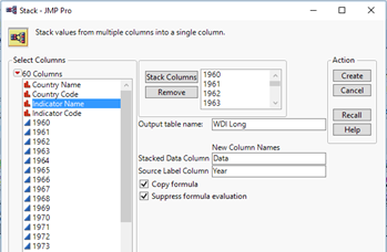
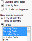
To achieve this we start with the Tables > Stack platform. As shown in Figure 7.15, we will stack all of the year columns from 1960 through 2015 into an output table called WDI Long. Name the data column Data and the new label column Year. In the lower left of the dialog, check Select under Non-stacked columns, and highlight the first three columns before clicking Create.

Figure 13: Specifications for the Stack Command

This will take a few moments and a window will open showing the progress of the operation. The new table should have five columns and 19,720,960 rows. For each country, every series appears 56 times now alongside the new Year column which runs from 1960 through 2015 repeatedly. From this table, we can split the data into a format in which most of the columns are different series, but first should make one adjustment.

The Columns panel in the WDI Long data table indicates that the new Year variable is nominal, as indicated by the red bars: . Now we want to treat the data series as separate columns.

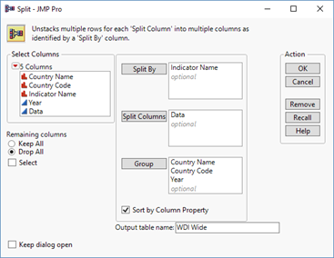
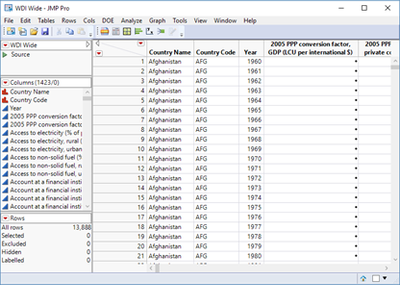
Select Tables > Split, and complete the dialog as shown in Figure 14. The indicator names will become the additional new columns, the cells will contain the numeric data, and observations will be grouped by country and year. This operation will also take a few moments, but when complete you will see the final data table with 1,423 columns and 13,888 rows (248 countries x 56 years). The resulting data table is shown, in part, in Figure 15.

Figure 14: The Split Dialog

Figure 15: The WDI Data Reshaped

Olympic Years Only

As noted above, this WDI table contains 56 years of data for each country. Going forward, we really only need those years that correspond to the summer Olympic which are held in years divisible by four. As with many tasks, there are multiple ways to accomplish this. Because of the modest scale of the task, I used the global Data Filter. First, I made sure that Year was Ordinal (unlike the image above), and then selected the years 1960, 1964 and so on through 2012. Granted we don’t yet have the 2012 medal counts (a task for another day to validate predictive models) but we’ll want the predictors from the WDIs.

Then, using Tables > Subset I created a new table for just the Olympic years. At this point, we have four JMP data tables to work with. Now the task is to merge them into one table for analysis. This is where the new Query Builder for Tables is a powerful, time saving addition.

Query Builder for Tables

New in JMP 13 is the ability to use Query Builder for JMP tables. Some readers might be familiar with this platform for ODBC and SAS data, introduced JMP12. We can now use it for tables already in JMP format.

Olympic Medals and Development Indicators

We can use Query Builder to assemble our table. Let’s suppose for simplicity that we want to extract some candidate explanatory variables from the WDI table, including the population, various wealth indicators, some measures of gender equity as well as measures of health like life expectancy. WDI offers numerous series that could be useful, but this will suffice for present purposes.

Recall the structure of each table. We have the Summer Olympics data since 1960 with one row per country per edition, and we have our wide form of the WDI data with 1,420 data series from 248 nations and country groups from 1960 through 2012. We also have the lists of IOC participating countries and the “crosswalk” table to match World Bank codes to IOC codes.

Query Builder allows us to choose multiple tables, indicate how to join them on shared columns, and then select columns and rows for inclusion in a final result table. We begin by choosing our four tables.

Tables > JMP Query Builder. This opens the Select Tables for Query (Figure 16) window. Make the WDI table the primary source, and choose the Country Codes, IOC codes and Medals by year & country as Secondary tables.

Figure 16: Select Tables for Query in Query Builder

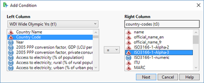
JMP can’t make a best guess about columns to join because there are no matching column names. In the secondary tables list, there are red X’s next to each table. We need to specify the matches. Click the Edit Join icon to the right of the top red X; the icon looks like a Venn diagram with two unshaded circles.

As shown in Figure 17, we first need to add the condition identifying the columns that will link the WDI table to the country codes table. Choose the matching columns and click Next.

Figure 17: Specifying Matching Columns for a Join

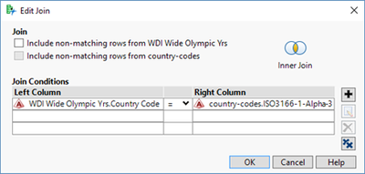
This opens the Edit Join dialog, (Figure 18) which does two important things. First, we can specify the type of join – inner, left outer etc. Second is permits more complex conditioning, such as joining on country plus year later. In the dialog at the top, uncheck the top checkbox to make this an inner join because we only want to include countries and not the regions included in the original World Bank data.

Figure 18: Tweaking the Join Specifications

We continue to incorporate the remaining two tables. When linking the medals and WDI tables we take care to create the compound join condition for countries and years. Once all joins are lined up, we go on to Build Query (see Figure 19).

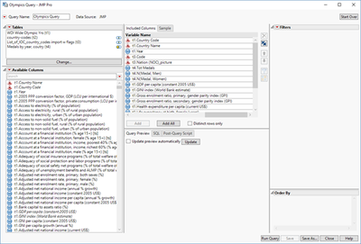
Figure 19: Choosing Columns for the Query

Give the query a meaningful name (like “Olympics Query”)

Working from the theory drawn from prior Olympic studies and understanding of the variables, choose relevant columns from the list of Available Columns. We might grab all columns willy-nilly and use an automated feature selection approach, but my preference here is to let the understanding of the context drive variable selection.

Run the query.

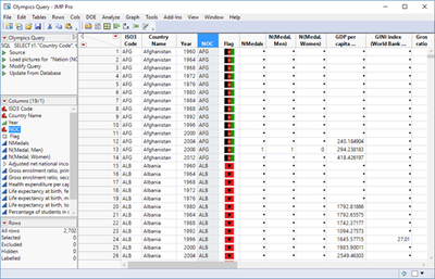
The result is a table with 19 columns and 2,702 rows – reflecting 14 years times 193 countries as shown in Figure 20.

Figure 20: The Result of Merging Four Tables

It is immediately obvious that there is a sizable issue of missing data here. Notably, in most years relatively few participating countries earn any medals at all. Because they were missing from the medalist table, those observations come in here as missing rather than 0’s. Moreover, many of the WDI observations are also missing for various reasons – though in those cases missing is decidedly different from zero. Before taking up the challenges of missing data and other hurdles, we’ll take a short digression to see another new data management feature in JMP 13.

Aside: Saving Memory with a Virtual Join

One disadvantage of joining tables is that we now have data values from the source tables actually replicated in the output table. With large datasets or particularly large data values (e.g. full-text or images), such duplication can be inefficient. JMP provides the alternative of a Virtual Join to temporarily access data from auxiliary tables by setting column properties to identify linked variables. We won’t work through this approach in detail as we did with Query Builder, but note it here because it is new and useful. In a virtual join, we don’t actually build a new table in memory. Rather, we identify linking columns that will function within different analysis platforms. For example, once we virtually join two tables, all of the columns in both tables appear in the list of columns available in (say) Graph Builder.

With a virtual join, we’ll want one (or more) main tables containing most of the crucial case-wise observations that will be important in the analysis as well as one or more referenced tables with linking columns consisting of unique, non-repeated values.

Consider the operation we have just completed. In this example, the WDI table was our primary data table and we had several secondary source which we joined them using different columns. The country ID code and Years appeared repeatedly in the WDI and medalist tables, but uniquely in the others. Our analytical focus will be on the numerical medal counts and development indicators, and the crucial information to be added from the other tables were the unique country codes and flags. Hence, the medalist and WDI tables will serve as main tables. These tables contain country codes that refer to information in the comprehensive country code and IOC countries tables. The latter two would be the referenced tables.

To establish a virtual join, we need to set two new column properties as follows.

In a secondary (referenced) table, open the Column Info for the unique key column. Click on Column Properties, and select LinkID near the very bottom of the list. Tagging this column as the LinkID basically identifies it as a primary key that can be referenced from another table.
In a main table, open the Column Info for the corresponding key column. Click on Column Properties, and select Link Reference. This opens a new panel asking for a Reference Table. Click Select Table and choose the referenced table from your directory.

In Figure 8.5 we see the two data tables after establishing the Link ID and Link Reference properties. In the referenced table there is a gold key next to the linked column name. In the main table, the same column is flagged as the referring column and below the list of available columns are additional accessible columns from the referenced table.

Now any analysis using the main table can make use of its columns as well as the columns from the referenced table. So, though this is not a literal join resulting in a new table it virtually joins the data from the two tables—without the added memory demands.

Combining Rows with Concatenate

We noted earlier that our data table omits the medal results from the London 2012 summer Olympics. Although I did not take this step for this project, it is a small matter to locate the results (Wikipedia has them), download the data table and either append it to the aggregated medals data using Tables > Concatenate or to merge it into the current set with Query Builder. In this way, one could eventually build a model using prior editions and test the accuracy of the estimates with 2012 results.

Initial explorations for Outliers, Missing data, and potential transformations

JMP users are probably familiar with the standard approaches to data exploration to find errors and unusual observations. This paper does not go into these issue in any depth, except to note several relevant JMP platforms:

Analyze > Distribution for a quick view of distributions, shapes, outliers and N missing
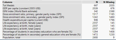
Cols > Column Viewer for numerical summaries. In Figure 21, we see where missing data is most prevalent.

Figure 21: Column Viewer Results (detail)

Analyze > Screening > Explore Outliers provides four different methods for identifying outliers in the data

For this presentation, I stopped short of a full analysis of strongly skewed columns but should mention that many of the variables here are indeed skewed. For example most nations have relatively low per capita wealth, with a very long right tail to the distributions. Before proceeding with imputation or modeling, we might well want to apply a log or other transformation. Because some variables are percentages and others dollar amounts, we might want to standardize columns. These are typical of the data preparation process, and JMP makes them easy to accomplish either within the data table or as a local transformation within an analysis platform.

Missing observations

We’ve seen that we have many empty cells in our combined table, and JMP offers several tools that can help us deal with them efficiently. Because the reasons for missingness vary and the demands of different projects differ, not all of the tools will be applicable here. The fact that we have panel data adds to the complexity since some of the automated tools are intended for cross-sectional samples. Still, the tools provide an efficient framework for coping with large numbers of missing observations.

There are a few reasonable starting points for this phase, but because I know in advance that the medals won column would contain numerous blanks, I chose to start there.

No Medals

The first group of missing cells are those in the medals column. These represent Olympic nations that won no medals in a given year. The quickest way to dispatch this issue is with Cols > Recode (now in the Cols menu in JMP13). Just go in and replace the missing values with 0.

What Else is Missing?

In the context of modeling, missing data can pinch us in multiple ways. For multivariable models, some methods require a full complement of observations row-wise. If the model for Y includes factors X1 and X2, we lose rows missing X1, X2 or both and this fact magnifies the impact of missing data. Tables > Missing Data Pattern identifies the number of rows for which all possible combination of columns are missing. The now-relocated Explore Missing Values platform can be very helpful in devising a strategy suitable for the project at hand. It is now in the Analyze menu among the Screening platforms.

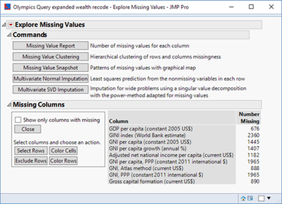
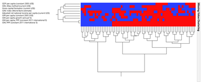
For this study, I actually went back and retrieved a total of 9 WDIs related to the wealth of the nations. Rather than explore all missing data at once, we’ll proceed in groups according to the main areas of size, wealth and gender equity. To illustrate, we’ll use the 9 wealth variables. Figure 22 shows the initial report on missing values for that group of columns. The information here is the same as the missing values shown earlier in the Columns Viewer output, though here we have additional columns.

Figure 22: Missing Value Report on Wealth Measures

If we then click on Missing Value clustering, we get a hierarchical graph of missing observations by column and row. Because it is a tall narrow image, I’ve rotated the view in Figure 22. Blue areas show where observations are present and red indicates missing observations. The idea in this diagram is to find groups of columns where missingness is least problematic and to know which rows are most impacted by missing data. While useful in its own right, it is particularly valuable if we decide to use one of the automated imputation methods that actually use different algorithms to replace blank cells with values. We’ll come back to that in a bit.

Figure 22: Missing Value Clustering

Informative Missing

In the modeling stage (which happily happens after this presentation) it can be helpful to identify some variables for which the very fact of missing data can itself carry meaning. For example, countries that do not collect or report figures on the proportion of girls enrolled in secondary education might not place a high priority on the education of female students. Among the column properties, we can tag a column as Informative Missing. When we later run an analysis that builds a model, the analysis platform makes use of missing and non-missing observations in its estimates.

Imputation

For some studies, it makes sense to impute missing values in a column based on either the column means or correlational patterns with other columns. As a simple example, if X1 and X2 covary reliably and (say) we have a value for X1 in row k but are missing X2, then why not estimate X2_k using the known value of X1 and the overall pattern of covariation in the rest of the data? This is the basic concept behind the automated imputation methods offered here. Rather than lose an entire row of data, we make a defensible estimate of what’s missing and proceed.

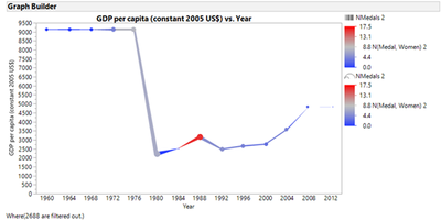
Before using these methods it makes sense to carry out transformations to standardize variables with different units of measurement and/or severe skewness. In this particular study, largely because of the repeated measures nature of the WDIs, I chose not to use the imputation offered by the Explore Missing Values platform. For example, many of the countries in the table are missing the per capita GDP values for the earliest years. The graph in Figure 23 illustrates the problem using Bulgaria, where 1980 was the first year for GDP to be reported. I used Multivariate Normal Imputation, combining GDP with some other wealth variables. The method replaced the first 5 years with the overall mean GDP for all countries, and in 1980 the actual values appear. In this graph, the size of the points reflects the total medals won and the coloration indicates the number won by Bulgarian women.

The point to be taken from this graph is that the imputation method does not produce a credible result here. Although we don’t know the correct values for 1960 through 1976, it is evident that should have been much close to $2,000 than $9000 for those years. A linear extrapolation or time-series approach would have been preferable, but less easy to accomplish at scale for all of the countries.

Figure 23: GDP per capita Imputed for Bulgaria

Conclusions

It is no secret that data preparation is often a particularly challenging and time-consuming phase of a project. JMP 13 adds several new capabilities centered on importing, managing, reconciling, and wrangling data. Because specific data management steps are intimately bound up with the needs of a particular investigation, this paper has described an illustrative study that required an assortment of data preparation tasks. The discussion is by no means comprehensive or exhaustive, but is typical of the types of problem-solving that consumes so much energy in the preparation phase of a study. The various inherent problems do present hurdles to overcome. One goal of the paper has been to show the ways in which JMP facilitates the process and speed up the “dirty work” of analytics.

REFERENCES

[1] Bernard, A and Busse, M. (2004) “Who wins the Olympic games: Economic resources and medal totals.” The Review of Economics and Statistics, February, 86(1): 413–417.
[2] Carver, R. (2014) Practical Data Analysis with JMP, 2^nd Ed., Cary NC: SAS Press.
[3] data.okfn.org (2016). Comprehensive country codes: ISO3166, ITU, ISO4217 currency codes and many more. http://data.okfn.org/data/core/country-codes.
[4] Hill, Eric. (2015). “Query Builder: The New JMP© 12 Tool for Getting Your SQL Data into JMP©”, available at https://www.jmp.com/content/dam/jmp/documents/en/white-papers/query-builder-jmp-12-107669_0515.pdf.
[5] JMP (2016), Version 13 Early Adopter Edition . SAS Institute Inc., Cary, NC, 1989–2013.
[6] McCormack, D. (2015) “It’s a dirty job, but somebody has to do it… Cleaning up data in JMP®”, JMP Discovery Summit 2015, San Diego CA.
[7] Reiche, D (2016) “Want more Olympic medals? Here’s what nations need to do to win” Washington Post, Aug. 3. https://www.washingtonpost.com/news/monkey-cage/wp/2016/08/03/want-more-olympic-medals-heres-what-na...
[8] Steinberg, Dan (2013) “How much time needs to be spent preparing data for analysis?” Blog post, June 19. http://info.salford-systems.com/blog/bid/299181/How-Much-Time-Needs-to-be-Spent-Preparing-Data-for-A...
[9] Wikipedia (2016) “List of IOC country codes.” https://en.wikipedia.org/wiki/List_of_IOC_country_codes.
[10] World Bank Group. World Bank Open Data. http://data.worldbank.org/.
[11] World Bank Group (2016). World Development Indicators. Highlights: Featuring the sustainable development goals. http://databank.worldbank.org/data/download/site-content/wdi-2016-highlights-featuring-sdgs-booklet....