- JMP User Community
- :
- JMP Discovery Summit Series
- :
- Past Discovery Summits
- :
- Discovery Summit 2015 Presentations
- :
- Use JSL to Scrape Data From the Web and Predict Football Wins!

- Subscribe to RSS Feed
- Mark as New
- Mark as Read
- Bookmark
- Subscribe
- Printer Friendly Page
- Report Inappropriate Content
William Baum (wjbaum), Graduate Statistics Student, University of New Hampshire
My project is one that uses JMP Scripting Language to pull data from multiple websites to predict professional football wins. The script automates an otherwise laborious process of collecting, aggregating and reorganizing data for analysis. Several sections of the script include different functions, such as cell processing to eliminate subscripts, and concatenation and joining of multiple data sets. An associative array is employed to compare the output of column formulas in separate rows. Finally, the results of multiple predictive models are compared. The purpose of this project is chiefly to illustrate the uses of JSL to automate the processes of data collection, organization and prediction, in a repeatable fashion.
Introduction
About two years ago, I learned that JMP could scrape data from the web with JMP Scripting Language [JSL]. As a graduate statistics student, I’m often looking for practice data on which to hone my analytical skills and improve my coding. It just so happens that I’m an avid American football fan and sports statistics are readily available online from many different sources. As an exercise, I attempted to predict total wins in a season for each professional football team, with data scraped from the web.
Data scraping and cleaning techniques can be applied to any data that are available in the form of html tables on the web. I find it amazing that JSL can be used to automate data clean up and perform modeling within a single script, or composite group of scripts. Furthermore, JMP helps those with limited programming experience, by enabling users to conduct an analysis through its graphical user interface [GUI], and afterward, to save the process as a script that can be reused. This saves users a lot of time when repeating analyses with updated or new data.
Set Up
The first step was to create folders in which to store the files that would be created during the process of data aggregation. I found that creating a folder for each data source worked well to organize the many files produced.
Next, I asked the script user to assign a local path for file storage, to make for cleaner code: dir = Pick Directory(“Select directory for file storage”, show files(0));
This local path can also be hard coded.
Once a path was selected, the data was then scraped from multiple websites and saved to individual files (one for each HTML table). These files were referenced later, during the data aggregation stage.
Scraping Data
With JMP, one must simply copy and paste URL names into the JSL code from a browser’s address bar. One may also put a link to the website directly in a script, which helps to open the website while editing JSL code: Web("http://url_name.com");
Importing Data
JMP has an assortment of useful tools to aid data import. First, one can attempt to save an html table as a JMP file, directly. This method works best when the data require little reorganization. The second method is to first save the html table as a comma separated value [CSV] file, which can then be imported to JMP with user-defined settings that are available through JSL. After looking at the imported table, I noticed several empty columns. Using the “delete columns” command, I was able to delete the empty columns from my table with a short script.
JMP automatically pulls the information from the web and saves the files. One doesn’t necessarily need to save these files, but data scraped from the web can be a bit messy at times. Saving data to a file makes for easier for debugging, because one can look at the imported tables and adjust the code, as needed.
Method 1
Data is imported and saved as a CSV file, initally:
ObjectName = Open(“http//:url_name1.com”, HTML Table(#))<< Set Name(“TableName1”) << Save(dir||“FileName1.csv”);
Method 2
Data is imported directly into JMP and saved:
ObjectName = Open(“http://url_name2.com”, HTML Table(#)<< Set Name(“TableName2”) << Save(dir||“FileName2.jmp”);
Cell Processing
When sorting character data in a script, even slight variations in imported strings can foul up your code. In this case, the playoffs were near and to indicate New England had clinched a division title, a “z” was inserted into their name. Thankfully, JMP offers a variety of commands to manipulate strings within cells.
In the following script, JMP loops through each row of the “Team” name column and deletes specified letters, if they appear in the beginning of the string. The “For Each Row” command makes for easy looping, which applies a process to each row. The conditional “if, then” phrase tells JMP what to do when the specific conditions apply. The “Contains” command returns the position of a specified item within the string. The “Substr” (substring) command returns part of the string: starting at a specified position, it returns the specified number of characters.
Combining Tables
Combining tables in JMP is easy through the “Tables” menu. The Tables menu offers multiple options. In general, I use “Join” to combine tables that have different columns, but the same row labels. I use “Concatenate” when I combine tables with different row labels, but the same columns. In this case, I concatenated information from multiple tables. One table had been created for each division of teams. Next, I sorted the rows of the resultant file by team name, alphabetically, to ensure like rows are matched during the joining process, later on.
Create a New Table
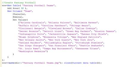
I find it useful to create a new table, prior to joining tables. JMP allows users to create a new table in a couple of ways. First, it can be done through the GUI. It can also be accomplished through a script. In this case, I used the “New Table” command to create a new table with the appropriate number of rows: one for each football team. I then added the column of team names with the “New Column” command, setting the values with a list.
Joining Tables
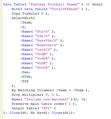
I find joining tables to be an annoying task without JMP. Thankfully, JMP has a nice GUI for joining tables in the “Tables” menu. Although naming conventions are always important, JMP automatically renames columns originating from different tables that share the same name. In this case, I joined the tables through the GUI, and then simply copied and pasted the table script of the resulting table into my larger, custom script. Otherwise, I would have had a lot of typing to do (renaming columns), prior to joining the tables. I repeated the join process many times.
Rename and Reformat Columns
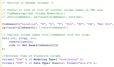
Once the joins were accomplished, I had a lot of odd-sounding column names. In order to eliminate confusion, I renamed those columns. To do so, I first created a list of preferred names. Then, I renamed the columns using the combination of a loop and the “Set Name” function.
Sometimes JMP imports data as a string, but the user needs a different column format, such as time. This is easy to change in the JMP GUI, but it can also be accomplished in a JSL script. In this case, I let JMP know that the column contained continuous time information, instead of character.
Reorganize Columns
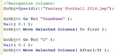
Once the data are aggregated and new columns are created, one may want to change the order of columns in the data table. It is easily accomplished in JSL with the “Move Selected Columns” command.
Data Table View
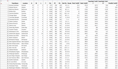
Here is a partial view of the completed data table.
Develop Associative Array
Once I finished aggregating the data, it was time to do some analysis. The first thing I wanted to compare was the relative strength of different teams, based on their strength of schedule, up to that point in the season. My goal was to predict how strong a team’s future performance would be, not only based on their own past performance, but also relative to their future opponents’ past performance. In order to do so, I had to compare information contained in cells located in different rows and columns of my table. Creating an associative array (a.k.a. dictionary, or hash map) was very useful for this task.
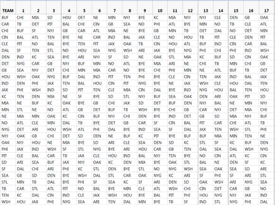
In JMP, one may use lists, matrices, or columns in an associative array. In this case, I used two columns, with a default value (null). The key column "TEAM" contained the abbreviated city names for each team. The value column, called “Strength”, was a formula column that calculated an index, combining wins & net points. I used each week (a column) of the 17-week game schedule as keys to reference the associative array values for that week.
17-week schedule: Keys
In the script, I defined the associative array, then I created a formula column to reference it. Again, the formula references the correct value through a subscript of the associative array, using the weekly opponent as the key. If the value in the key column is not in the associative array, the function returns a null value (works well with bye weeks in the schedule).
I then created a new column for each week to compare team strength. These two formulas could have been joined, but I preferred to keep them separate so I could visualize the different metrics in the data table.
Next, I counted the number of predicted wins for the season. A simple way to count the column results was to create a new formula column that contained the sum of a series of “If-Then” conditions for each of the 17 columns. In this case, if the difference in Strength was positive, the prediction was considered a win and counted.
Create Prediction Models
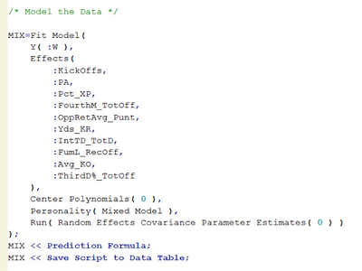
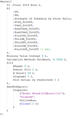
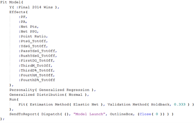
JMP has a variety of modeling techniques for prediction. Many techniques are accessed through the “Analyze” menu, including the “Fit Model” and “Neural” platforms. When creating a custom script, I recommend developing optimal models in JMP’s platforms, first. Then one can save the model script to the data table (through the GUI), and copy and paste the code into the custom script. One may also use JSL to save model scripts to a data table. This gives users the flexibility to set the model to run automatically, or to make the model available in the list of data table scripts of the table created by the custom script.
Here is one example.
Advanced Modeling Techniques in JMP Pro
Several advanced modeling techniques are available in JMP Pro, which are not available in the standard version of JMP. Two examples are the boosted version of the neural net, and the elastic-net generalized-regression technique. Another nice quality of JMP is its ability to perform holdback validation with a user-specified proportion, automatically selecting a random sample from a dataset. This eases both validation, and model comparison.
Boosted Neural Net
Elastic Net
Sometimes, the average of multiple model predictions may outperform individual model performance.
Here I created a formula column in JSL that averages two prediction formulas.
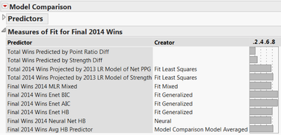
JMP Pro has a model comparison platform, in which users can compare the relative effectiveness of multiple models, side by side. The model comparison platform also gives users the power to average multiple models together, with just a few clicks.
Model Comparisons
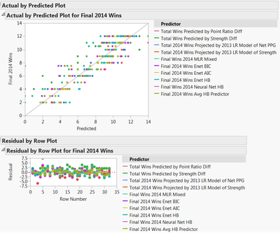
In this case, the average of the Neural Net and Elastic Net models (with holdback validation [HB]) performed slightly better than either of the two individual models, alone. Another nice feature of the model comparison platform are "actual by predicted" and "residual by row" plots.
Model Comparison Plots
Conclusion
With JMP Scripting Language [JSL], JMP can scrape data from multiple web sources, process the data, perform multiple predictions, compare them, and display them– all within a single script. The effective use of JSL can save a lot of time, especially when one must repeat an analysis on a regular basis.
Discovery Summit 2015 Resources
Discovery Summit 2015 is over, but it's not too late to participate in the conversation!
Below, you'll find papers, posters and selected video clips from Discovery Summit Europe 2015.
- © 2024 JMP Statistical Discovery LLC. All Rights Reserved.
- Terms of Use
- Privacy Statement
- Contact Us


